Geological Survey Professional Paper 1033 The Structure of the Olympic Mountains, Washington—Analysis of a Subduction Zone

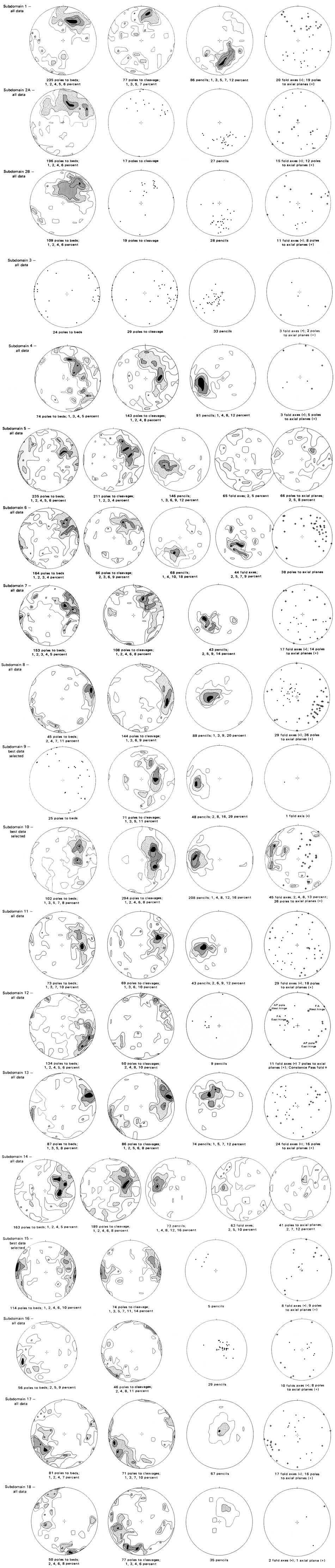
FREQUENCY DIAGRAMS FOR SUBDOMAINS

Frequency diagrams for subdomains shown on figures 25 and 26. Contours drawn by hand on percentages calculated and plotted by computer to nearest whole number; contours shown to lower right of each diagram. All percentages calculated per one percent area. Data not contoured if less than 40 points.

(click on image for an enlargement in a new window)

COMPUTERIZED STRUCTURAL DIAGRAM PROGRAM

In order to handle the large amounts of complex structural data obtained while mapping the Olympic Mountains, we established a two-part computer program in Fortran IV. The first part allows storage of the structural data on punchcards with provisions to select the data by type and geographic location subdomain). The second part of the program prepares a pole-density orientation diagram from the selected data. The computer program for pole-density orientation diagrams was made at the University of Alberta by Muecke and Charlesworth 1966). Our orientation program deck is a duplicate of the Canadian deck, lent to us by Dr. Charlesworth. Ming Ko, of the U.S.G.S. Computer Center, modified the Canadian program for our needs.

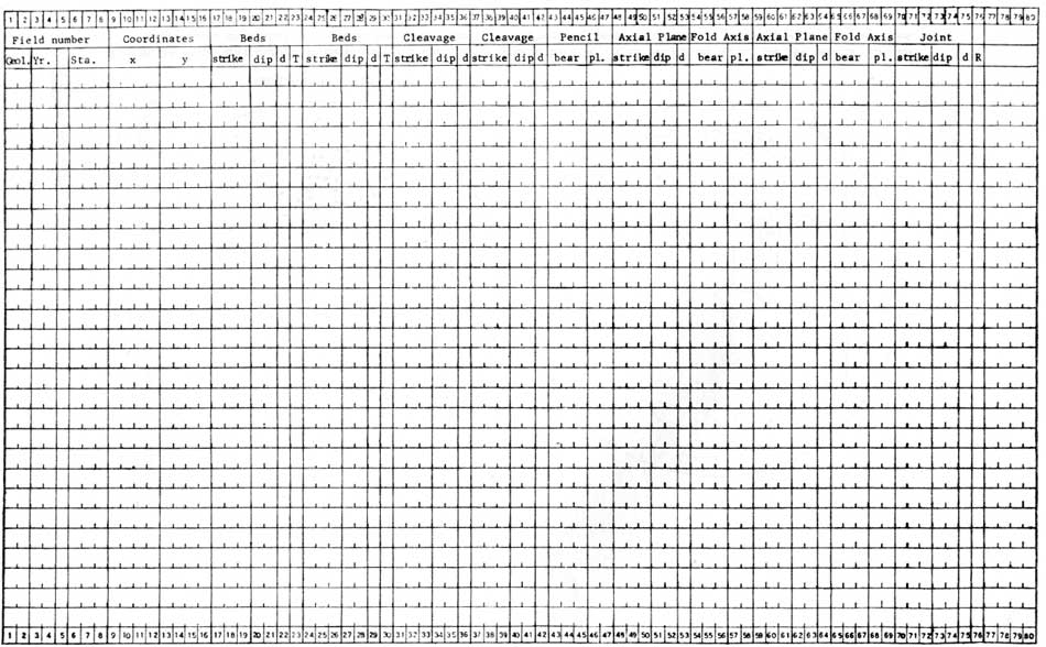
The storage of data was facilitated by the use of forms (fig. 33) that we filled out in the field. Any type of line or plane can be entered on the form and treated by the program. We measured dips to the nearest 5°, strikes to the nearest 2°. Before the data were entered on punch cards, station coordinates were punched by use of a coordinatograph.

Figure 33.—Computer form for structural data.

The program allows subdomains to be selected by coordinates and (or) indicated stations. If coordinates are used, each subdomain is outlined as nearly as possible by two rectangles, specified by their southwest and northeast corners. Stations can be added or subtracted individually to fill in irregular subdomains.

Because the Olympic rocks are particularly prone to sliding and slumping (see Tabor, 1971), we included an option of select data on the basis of field observation of reliability, a somewhat subjective judgment. We found that the results for all data and for only the best data were about the same. Most subdomains were run with all the data.

The following summary of the pole-density orientation program is modified from a description of the program by H. A. K. Charlesworth (written commun., 1967).

The program counts out points on the reference sphere, not on their projection in the equatorial plane. The pole densities obtained are then projected onto the equatorial plane and faithfully reflect the true pole densities.

The computer converts the strike, dip. and direction of a plane to the bearing and plunge of the normal to the plane. All the bearings and plunges are then changed into direction cosines of unit length.

The counting out of the poles in the reference sphere is accomplished by the use of a circular cone with semivertical angle, the value of which is determined by the percentage of the total area of the projection that the counter is required to cover. The percentage of the total area counted and the number of counting locations are chosen such that the counting cones overlap so as to assure that all points on the sphere are counted. At the same time, the counting area is kept small in order to obtain the best possible definition of any differences in the densities of the points.

The number of data readings in each data set falling within the counting cone at each counting locality is converted into the percentage of the total number of points processed.

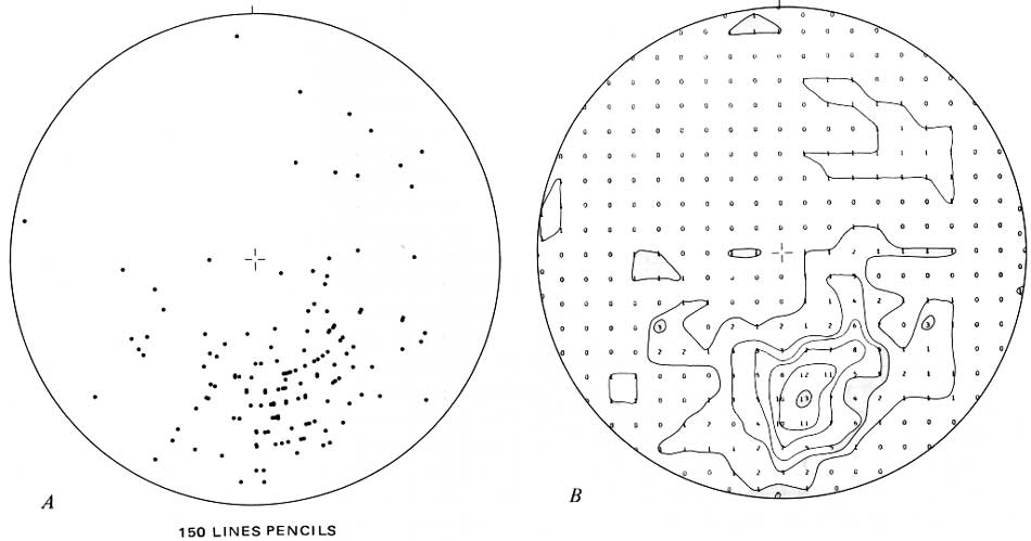
In order to facilitate a simple output format for a line printer, the counting locations were chosen to form a regular grid and projected from the lower hemisphere of the reference sphere onto the equatorial plane by equal-area projection fig. 34B). For the convenience of accurate contouring, these locations were augmented by 14 additional points near the periphery of the projection. We contoured the printed densities by hand; a subprogram that plots the projections of the pole intersections (fig. 34A) was especially useful in subdomains with small amounts of data.

Figure 34.—Computer output for structural program. Circles reduced from 10 inches. A, Plotter output for 10 pencils. Circular alinement is an artifact of recording dips to the nears 5°. B, Frequency plot of same data in percentages per 1 percent area. Contoured by hand. (click on image for an enlargement in a new window)

In keeping with the spirit established by Muecke and Charles worth, we maintain a program card deck with our modifications (data retrieval and plotting subroutine), available for loan and duplication. Address inquiries to R. W. Tabor, U.S. Geological Survey, 345 Middlefield Road, Menlo Park, Calif. 94025.