Geological Survey Professional Paper 1365 Ice Volumes on Cascade Volcanoes: Mount Rainier, Mount Hood, and Mount Shasta

The comparatively extreme electrical resistance and homogeneous nature of ice has allowed successful radar sounding through several miles of polar ice (Fitzgerald and Peran, 1975, p. 39). Until recently, similar success had eluded researchers in their efforts to sound temperate glaciers (glaciers having ice at the pressure melting point). The main problem encountered is the scattering caused by water found in temperature glaciers, not the increased electromagnetic absorption in the ice due to higher temperatures. Thus, the signal-to-noise ratio cannot be increased by improving system performance (Smith and Evans, 1972, p. 133). The ratio of radio wavelength to effective scatterer radius is recognized to be the controlling factor, and theoretical analysis shows that, if scattering is to be brought down to an acceptable level, the frequency must be reduced to 5 MHz or lower (Watts and England, 1976, p. 46).

Conventional radio detectors are tuned receivers, measuring a rectified electric field at a single frequency as a function of time. Therefore, several cycles of the carrier frequency need to be received in order to generate a response. As a frequency of 5 MHz corresponds to a wavelength of more than 100 ft, this resolution is inadequate for many temperate glaciers.

In theory this problem can be circumvented by use of a monopulse source at the correct frequency and an untuned receiver, which measures an unrectified electric field as a function of time. In this way, arrival times of the reflected wave could be picked within the accuracy of a small fraction of a single cycle (Watts and England, 1976, p. 40).

The technical breakthrough in application of these ideas was achieved by Roger S. Vickers and R. Bollen (1974, p. 2) and tested by them at South Cascade and Columbia Glaciers. Nondestructive avalanche transistor transmitters provided the necessary monopulse, and resistively loaded antennas eliminated the resonance problem (Watts and England, 1976, p. 40). Subsequent refinements resulted in the portable field unit used in this study.

APPLICATION

A thorough treatment of a similar system has been published (Watts and Wright, 1981), so only a basic outline of the instrument circuitry is provided, except where differences merit detail.

The principal components of the ground-based monopulse radar are schematically depicted in figure 24.

FIGURE 24.—Schematic diagram of the radar system used in this study (Kennard, 1983).

The two power supplies consist of 12-volt, rechargeable battery cells with gelatinized electrolyte. Of the two main parts, the receiving oscilloscope has the heavier power requirement, but in no instance was more than one battery change in a working day needed.

The specific transmitting circuitry was designed by David Wright, modified by Steven Hodge, and built by Robert Jacobel under the auspices of the Geological Survey. Circuit diagrams are available from the Geological Survey's Project Office—Glaciology. The antenna design was done by G. C. Rose and R. S. Vickers (1974, p. 261) and modified for field use by Steven Hodge (U.S. Geological Survey, written commun., October 1978).

The transmitting power supply energized a trigger circuit and a high-voltage direct-current source. The trigger controlled the repetition rate (as distinct from the frequency) of the transmitted monopulse. This rate was variable over two ranges, 0.1 to 12.8 kHz. The oscilloscope recorded both the transmitted (air) wave, returns from intraglacial scattering, and the reflection from bedrock. Thus, the repetition rate needed regulation so that a subsequently transmitted wave would not obscure an earlier reflected wave.

The brightness of the oscilloscope trace is proportional to the repetition rate, which is an important factor in a sunlit field situation. Power consumption was increased with higher pulse rates but still never approached that of the receiver. A repetition rate of 10 kHz was generally used.

The power supply was a low to high voltage converter that supplied the necessary power for the transmitted pulse. A 750-volt, 20 mA capacity converter sufficed for the pulse generator configuration at the repetition rates used.

The pulse generator consisted of a variable number of avalanche transistor stages. Increasing the number of stages increased the amplitude of the transmitted pulse, until it was limited by the high-voltage supply and the thermal-dissipation capabilities of the transistors. Three configurations were tested: low power (2 stage), medium power (3 stage), and high power (4 stage). The optimal unit for these studies seemed to be the medium power pulse, which produced 600-volt pulses into a 50-ohm load. The low-power unit produced approximately 40 percent less power (Jacobel and Raymond, 1984) but caused no problem when used in the field. The high-power unit did not produce significantly more output but did draw more current.

When a stage avalanched, it produced a fast voltage rise time (several tens of nanoseconds) and then returned to a high impedance state. The discharge current was limited by the antenna impedance, so the avalanching was nondestructive.

The final component of the transmitter system was the resistively loaded antenna, which was identical to the receiving antenna. The center frequency of the transmitted pulse (limited by the pulse generator) is a function of the antenna length and a resistive loading constant (ψ). When the antenna is lying on an ice surface, the frequency is given approximately by the equation

where v is in megahertz and l' is the antenna half length in meters.

To prevent ringing of the pulse produced by the transmitter the antenna is loaded according to the relation

where R is resistance per unit length at distance x from the feed point, and ψ is a constant in ohms. The constant, ψ, affects the pulse duration and the radiated power. Increasing ψ decreases the duration of the pulse (increasing resolution) but also decreases the radiated power. In practice, the variation is not critical, and in applications where increased power is needed, such as in thick ice, the decrease in resolution is usually acceptable.

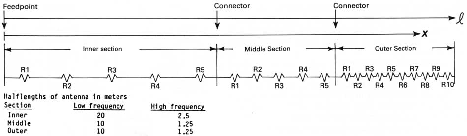
The two main criteria for antenna design are the length, which determines frequency, and the resistive loading, which determines resolution and power. In this study, two basic configurations were chosen with respect to frequency: the high and the low. Because frequency is a function of antennas length only, it can be changed by simply removing or adding center sections of the antenna. If the section lengths are chosen as shown in figure 25, only 10 discrete resistor values are required for a given ψ value, and one antenna design is thus capable of producing pulses at six different frequencies (Steven Hodge, U.S. Geological Survey written commun., October 1978).

FIGURE 25.—Diagram of antenna illustrating positioning of resistors in the radar antenna. (Diagram from written communication, S. M Hodge, U.S. Geological Survey, October 1978). To determine the required values of resistors in the outer antenna section, the antenna is divided into 10 intervals. Resistance is calculated where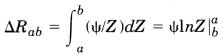 Z = l - x, where l is the antenna half-length, and x is the distance from the antenna feedpoint. R values for the inner middle sections equal values for R 1 through R 5 in the outer section. Half-lengths for high and low frequency antennas are also shown. (click on image for an enlargement in a new window)

The antennas used on the project were ψ = 400 Ohm (low frequency) and ψ = 1,500 Ohm and 2,500 Ohm (high frequency). In testing antennas, it has been found that the outer arms alone (10 m, 5 MHz) of the low frequency antennas give the best results on the relatively thin, temperate glaciers of the Cascade Range and were the easiest to operate. These tests were not comprehensive, yet it was found that if a good bottom reflection could not be achieved with the low-frequency set, it could not be achieved with the high-frequency set. This result was not surprising, considering the expected signal scattering in temperate glaciers. Generally, in this study the 400-ohm antennas were used.

The transmitted signal was about 106 times stronger than the received signal, necessitating the use of separate but identical antennas. The receiving antenna impedance was matched to the oscilloscope with a balun. Optimal input:output voltage and impedance ratios (Hodge, U.S. Geological Survey, written commun., October 1978) were found to be 3:1 and 9:1, respectively. Others have also used a preamplifier (for thick ice) and a bandpass filter (1-10 MHz) at this stage (Watts and Wright, 1981, p. 460), though these were not required in this fieldwork.

The oscilloscope constitutes the core of the receiving system. A bandwidth of 30 MHz is used, and the unit is otherwise chosen according to power requirements, weight, sensitivity, and trace brightness.

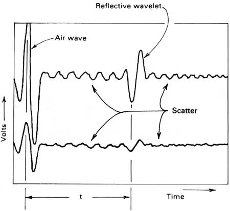
The oscilloscope trace is triggered by the incoming air wave and records this wave and the reflected wavelet (fig. 26). A two-channel oscilloscope is preferable because the incoming signal can be viewed at two different amplification levels. In this way, a relatively strong air wave and a reflected wave can be viewed in detail simultaneously.

FIGURE 26.—Oscilloscope output. Air wave and reflected wavelet as seen on the oscilloscope screen. Quick-developing photographs were taken at the traces at each measurement point. The time interval between wave transmission and receival is expressed as t. Two traces were set at differing amplitudes to accent features in the air wave and the reflected wave.

The trace output was recorded by an oscilloscope camera on self-developing film. Minimizing light leaks and maintaining the film at higher-than-ambient temperature were the only difficulties encountered.

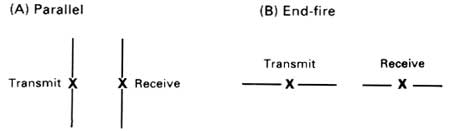
The layout geometry of the antenna at each measurement point depended on the ability of a particular configuration to give an unambiguous bottom return. Figure 27 shows the primary antenna layouts used on the glacier. In general, the parallel configuration (A) was tried first. The air-wave used to trigger the scope is of predictable polarity and there is maximum coupling of the antennas. An attempt was made to align the antennas parallel to the expected bottom contours. If ambiguous returns continued, the separation distance between the transmitter and receiver antenna was changed.

FIGURE 27.—Typical antenna configurations used during measurements. Placement was dependent on the clarity of a bottom return on the oscilloscope trace.

If bottom returns were still unsatisfactory, the end fire configuration (B) was used at various separations. Although the airwave coupling is decreased, the quality of bottom returns would occasionally be enhanced.

The obtaining of some successful bottom returns even with both or parts of the antennas hanging down crevasses, and, in one instance, coiled, indicates that the antenna configuration was not critical. The presence of surficial debris, crevasses of various orientations, water, or volcanic ash did not seem to have any effect on the success of receiving bottom returns. In general, if a satisfactory bottom return was not found in an area, it was necessary to move at least an antenna-length away from the original measurement location.

As the air wave triggers the oscilloscope, it is necessary to know the transmitter-receiver separation in order to determine the total travel time of the reflected wave. First seen on the left side of the scope trace is the air wave.

A surface wave also travels directly through the ice and usually appears as a minor disruption of the air-wave. Next are returns of scattered signals from ice inhomogeneities, finally followed by the reflected wave, which has undergone a phase reversal.

For depth determination, the information of interest is the time delay (t) between a point on the airwave and a corresponding point on the reflected wave. Because frequency is not necessarily preserved between the air and reflected waves, it is most accurate to choose this point to be early along the pulse. Almost exclusively the first peak was chosen (whether of positive or negative amplitude) to be the basis for calculation of the time delay.

For purposes of this study, the only concerns were the respective positions of the air and reflected waves. It is possible that useful information about the nature of englacial scatterers can be obtained from further study of the remainder of the recorded signals (Jacobel and Raymond, 1984).