|
PECOS
From Folsom to Fogelson: The Cultural Resources Inventory Survey of Pecos National Historical Park |

|
CHAPTER 6:
SETTLEMENT
Karl K. Benedict and Janet D. Orcutt
Site locations have the potential to provide insight into community development in the Pecos area. Decisions about where to build a structure or conduct activities reflect the exploitation of critical resources, including wild plants, fauna, agricultural land, and nonfood raw materials. They also reflect knowledge about past activities in the area, the current activities of other people in the area, and the nature of one's relationships with those people. This chapter explores these aspects of settlement through a variety of approaches. In the first part of the chapter, the Palmer Drought Severity Index (PDSI) is used to characterize potential agricultural productivity in each period, and this information is used to generate expectations for site locations. These expectations are evaluated using information recorded by survey crews on site elevation, landform, and modern vegetation. In the second section of the chapter, the effects on site placement of the changing social and economic relationships accompanying aggregation are explored through nearest-neighbor distances between site types. In the last part of the chapter, the relationships between site location and localized resources are examined in sharper detail using plant productivity potentials for soils derived from a recent soil survey in Pecos National Historical Park. Throughout the chapter our expectations for site locations relative to the physical and cultural landscape differ according to the general activities expected at each site type (see Chapter 5).
Characterizing Climate through the Palmer Drought Severity Index
The pueblo period occupants of the Pecos area grew corn and other domestic crops and also depended heavily on hunting large game and gathering wild plants for their subsistence (Cordell 1998; Kidder 1958). The population's ability to meet subsistence needs, therefore, depended first on the nature of climatic variability.
Certain aspects of prehistoric climate are important in understanding how the agricultural subsistence system at Pecos functioned and the problems that farmers faced. Climatic changes affecting agricultural productivity should influence locational decisions, especially with regard to field houses (seasonal sites) and habitations where agriculture may take place. The PDSI is one way to estimate climatic stress on crops (Rose et al. 1982), because it is a rough measure of the moisture available to plants during the growing season. The PDSI, which is "an index of meteorological drought, as opposed to a specific biological or hydrological measure" (Rose et al. 1982:109), is calculated using estimates of potential evapotranspiration and is based on tree-ring indices.
The mean and variance of the PDSI have been used to examine potential agricultural productivity in other areas of the Southwest and are especially useful for characterizing local conditions when time periods are relatively short (Kohler and Van West 1992; Orcutt 1999b). The mean, in particular, is not helpful in characterizing lengthy time spans however, because it over-simplifies a great deal of variability. Because the time periods developed for the Pecos survey are long (see Chapter 4), we created a dryness index for the PDSI for Periods 2-5 (A.D. 1200-1700) that transforms the PDSI values into an ordinal scale. The annual PDSI values and classes were transformed according to the following: 0 is normal/wet, 1 is dry, and 2 is very dry (Table 6.1). Five-year moving averages were calculated for each year. We chose to calculate five-year moving averages for each year because if people rely on two to three years of storage to help them through dry periods, as is known for Pueblo groups in the southwest, five drier years most likely would stress the storage system and invoke adaptive responses.
| Table 6.1. Palmer Drought Severity Index values
and dryness index. | ||
| PDSI Value | PDSI Class | Dryness Index |
| > 3.99 | Extremely wet | 0 |
| 3.00 to 3.99 | Very wet | 0 |
| 2.00 to 2.99 | Moderately wet | 0 |
| 1.00 to 1.99 | Slightly wet | 0 |
| 0.50 to 0.99 | Incipient wet spell | 0 |
| 0.49 to -0.49 | Near normal | 0 |
| -0.50 to -0.99 | Incipient drought | 1 |
| -1.00 to -1.99 | Mild drought | 1 |
| -2.00 to -2.99 | Moderate drought | 2 |
| -3.00 to -3.99 | Severe drought | 2 |
| < -3.99 | Extreme drought | 2 |
The median dryness index is 0.4 for each period, and Period 2 (A.D. 1200-1325) has the widest range of values. Periods 3 (A.D. 1325-1450) and 4 (A.D. 1450-1575) are similar except for one outlier (drier) year (A.D. 1425) in Period 3. Variability is lower in Periods 3 and 4 than Period 2. Period 5 (A.D. 1575-1700) is more normal/wet than the others, but several dry years are outliers—1587, 1601, 1602, 1667, 1669, and 1671—and extreme outliers—1583, 1668, and 1670. The general trend in the index over time is toward more normal/wet conditions.
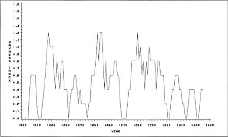
Dry periods are considered to be any number of consecutive years corresponding to the median dryness of 0.4 or greater. The following are the extended dry intervals in Period 2 (A.D. 1200-1325) (Figure 6.1): 1215-1231, 1234-1240, 1248-1267, 1274-1298, 1304-1310, and 1316-1319 (mild). The dry periods average more than 13 years in duration, and approximately one quarter of the indices are 0.8 or larger, which is towards the dry end of the scale. The actual yearly PDSI values, not the dryness index, indicate high variability associated with wide swings above and below normal between 1270 and 1298. Slightly less variability characterizes the 1240-1265 interval.
|
| Figure 6.1. Palmer Drought Severity Index dryness index for Period 2 (A.D. 1200-1325). |
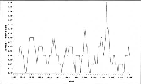
There are more dry periods in Period 3 (A.D. 1325-1450) (Figure 6.2), seven rather than six, but the average of nearly 11 years is slightly shorter than the average in Period 2 (A.D. 1200-1325). The dry periods are 1324-1331, 1336-1356, 1360-1370, 1377-1386, 1390-1394 (mild), 1397-1403, and 1415-1428. Fifteen percent of the annual indices are 0.8 or greater, 10 percent fewer than Period 2. The yearly PDSI values indicate much less variability than Period 2.
|
| Figure 6.2. Palmer Drought Severity Index dryness index for Period 3 (A.D. 1325-1450). |
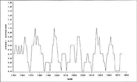
The eight dry periods in Period 4 (A.D. 1450-1575) (Figure 6.3) average approximately 10 years and occur during the years 1445-1465, 1471-1484, 1495-1501, 1506-1510 (mild), 1516-1520, 1523-1528, 1542-1553, and 1558-1566. Twelve percent of the indices are greater than or equal to 0.8. The yearly PDSI values indicate fewer very wet years and more very dry ones than in Period 3 (A.D. 1325-1450).
|
| Figure 6.3. Palmer Drought Severity dryness indexx for Period 4 (A.D. 1450-1575). |
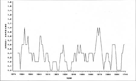
There are ten dry periods in Period 5 (A.D. 1575-1700) (Figure 6.4), but they are shorter than those in previous periods, averaging approximately seven years. The extended dry periods are 1573-1577 (mild), 1579-1591, 1600-1605, 1608-1610 (mild), 1625-1629, 1644-1652, 1658-1673, 1678-1680 (mild), 1685-1689, and 1696-1699. Only seven percent of the indices are greater than or equal to 0.8. There are no wide extremes in the yearly PDSI values until late in the period, approximately 1680-1700. Drier spikes in PDSI values are not as severe as previous periods, and there are many very wet years. Overall, from Period 2 (A.D. 1200-1325) to Period 5 there is a trend towards shorter but more frequent dry periods.
|
| Figure 6.4. Palmer Drought Severity Index dryness index for Period 5 (A.D. 1575-1700). |
Expectations for Site Locations
This characterization of the rainfall regime elicits a series of expectations for site locations through time. In subsequent sections of this chapter expectations for the diversity of site locations will be tested using site environment information recorded by the field crews, and a nearest-neighbor analysis is used to examine the social influences on site locations and the distances between sites. In addition, decisions concerning site placement will be further explored through the relationship between the potential productivity of local soils and the location of different site types.
Extended and frequent dry periods should affect agricultural yields, which, in turn, affect people's choices for site locations. This is true especially for habitation and seasonal sites where we expect agriculture to occur. Depending on the levels of stress experienced during dry periods, people may locate sites to avoid conflict with their neighbors over scarce arable land. Period 2 (A.D. 1200-1325) appears to be the most variable, and it is drier than the others. To cope with the variability, we expect sites in diverse settings, which would provide a range of subsistence options that could be used depending on the conditions in a particular year. Because there are few habitation sites in Period 2, there should be a number of locational choices available. Competition, which is indicated by regular spacing between sites, is not expected in Period 2.
The unpredictability and dryness in Period 2 (A.D. 1200-1325) disappear in Period 3 (A.D. 1325-1450), which may be the best prehistoric climate period. Because climate appears to improve in Period 3, agricultural production should be more predictable and reliable. We expect diverse site locations in Period 3 because the number of sites increases. If the increase in sites also indicates that more people are using the landscape, we expect competition over land to arise, and so more regular spacing between sites.
The dryness index suggests that Period 4 (A.D. 1450-1575) is similar to Period 3 (A.D. 1325-1450). The annual PDSI values, however, show more very dry years and fewer very wet years than Period 3. We know there are fewer sites in Period 4 and that Pecos Pueblo is the dominant habitation. Site locations may reflect several things, including the presence of the large aggregate at Pecos Pueblo, climate and agricultural productivity, and interactions with neighbors. By Period 4, land and resources had been exploited for over 200 years, and it may be necessary for people to go farther to find suitable arable land and wild resources. Concentrating people in one location also forces them to farm and forage farther from the main pueblo. We expect smaller sites to be located away from Pecos Pueblo.
Period 5 (A.D. 1575-1700) appears to be the least dry period. The annual PDSI values indicate that the widest annual extremes primarily occur between A.D. 1680 and 1700, the period of the Pueblo Revolt and Reconquest. Drier spikes in the annual values are less severe than in previous periods, and there are numerous very wet years throughout Period 5. It is likely that Pueblo land use during Period 5 is affected by factors other than climate, however, so our expectations may not be valid for the seventeenth century. Pecos Pueblo remains the dominant habitation, but the Spanish mission is built nearby, using pueblo labor and supplies, and requiring pueblo labor for its maintenance. In addition, the Pueblo Revolt and the Reconquest also occur during this period. We expect people to continue farming and foraging at a distance from Pecos Pueblo, and nearest-neighbor distances should indicate that residents in other habitation sites avoid locating close to Pecos Pueblo. Seasonal sites should be situated in good agricultural areas, and we expect special-use sites to be in a diversity of locations to exploit wild plants, fauna, and nonfood raw materials.
Site Types by Environment
To test these expectations for site location based on the characterization of climate, we examine the distributions of site types relative to several environmental variables for Periods 2-5 (A.D. 1200-1700). Use of the area was light and sporadic in Periods 0 (pre A.D. 1075; number of sites=3) and 1 (A.D. 1075-1200; number of sites=2), and there are so few sites that we can not identify trends or patterns in locations. We also do not discuss Period 6 (post A.D. 1700) because the period is so long and encompasses many cultural changes.
The analyses rely on the following variables recorded by the survey crews: elevation, landform, and vegetation. The numerous vegetation types used by the survey, however, are grouped into Sivinski's (1995) four vegetation communities—grassland, riparian, piñon-juniper woodland, and mixed conifer forest—and combinations of those communities. The placement of the different site types in each period is first discussed, then changes in each site type over time are presented.
Period 2 (A.D. 1200-1325)
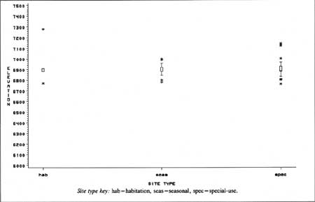
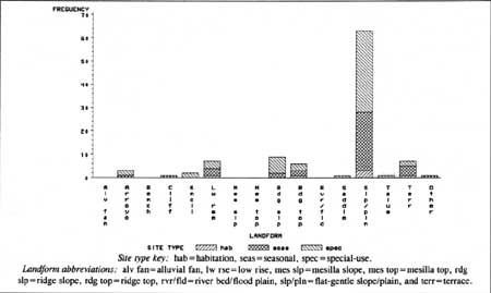
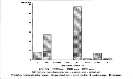
Five of the habitations occur between 6,770 and 6,910 ft (2,063 and 2,106 m) in elevation. The sixth one is at 7,280 ft (2,219 m) (Figure 6.5). Half of the habitations are on a flat-gentle slope/plain, and one each is on a ridge top, a low rise, or a terrace (Figure 6.6). Habitations are associated with piñon-juniper woodland and grassland vegetation (Figure 6.7).
|
| Figure 6.5. Box plot of elevation (in feet) by site type for Period 2 (A.D. 1200-1325). |
|
| Figure 6.6. Frequencies of each site type by landform types in Period 2 (A.D. 1200-1325). |
Although seasonal sites (n=39) are more numerous than habitations (n=6), they occur in a smaller elevation range, extending from 6,780 to 7,000 ft (2,067 to 2,225 m) (Figure 6.5). Approximately 67 percent of the sites are between 6,860 and 6,920 ft (2,091 and 2,109 m). Most seasonal sites are on a flat-gentle slope/plain, but seven other landforms also are used (Figure 6.6). Seasonal sites are associated with more vegetation communities than habitations; however, nearly 70 percent are found in piñon-juniper woodland (Figure 6.7).
|
| Figure 6.7. Frequencies of each site type by vegetation community for Period 2 (A.D. 1200-1325). |
Special-use sites (n=56) cover a slightly greater elevation range than seasonal sites, extending from 6,760 to 7,140 ft (2,060 to 2,176 m). There are three clusters or concentrations of sites. The largest group, 41 percent of the sites, is between 6,850 and 6,880 ft (2,088 and 2,097 m); the second group comprises 20 percent of the sites and is between 6,900 and 6,920 ft (2,103 and 2,109 m), while the third group, 14 percent of the sites, is between 6,960 and 7,000 ft (2,121 and 2,134 m) (Figure 6.5). Several landforms are represented in special-use site locations. The most common is a flat-gentle slope/plain, and eight others also are occupied (Figure 6.6). Special-use sites occur in several vegetation communities, although 70 percent of the sites are in piñon-juniper woodland or a combination of grassland and piñon-juniper woodland (Figure 6.7).
Period 3 (A.D. 1325-1450)
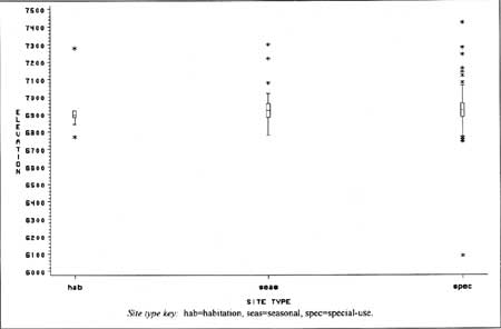
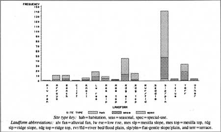
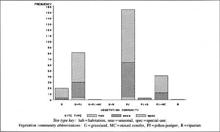
Habitations (n=10) occur between 6,770 and 7,280 ft (2,063 and 2,219 m) in elevation; however, 70 percent are in a band between 6,880 and 6,920 ft (2,097 and 2,109 m) (Figure 6.8). Habitations are found on seven different landforms, although 40 percent of them are on a flat-gentle slope/plain (Figure 6.9). Ninety percent of habitations are in piñon-juniper woodland and grassland/piñon-juniper woodland (Figure 6.10).
|
| Figure 6.8. Box plot of elevation (in feet) by site type for Period 3 (A.D. 1325-1450). |
|
| Figure 6.9. Frequencies of each site type by landform types in Period 3 (A.D. 1325-1450). |
|
| Figure 6.10. Frequencies of each site type by vegetation community for Period 3 (A.D. 1325-1450). |
Seasonal sites (n=104) cover a slightly larger elevation range than habitations, from 6,780 to 7,300 ft (2,067 to 2,225 m), and are most common between 6,880 and 6,960 ft (2,097 and 2,121 m) (Figure 6.8). Seasonal sites occupy a variety of landforms, although a flat-gentle slope/plain is predominant (Figure 6.9). Seasonal sites are in a greater diversity of vegetation communities than Period 2 (A.D. 1200-1325), which goes along with almost triple the number of sites. Piñon-juniper woodland and grassland/piñon-juniper woodland remain the most common communities, but there is an increase in locations associated with piñon juniper woodland/mixed conifer forest (Figure 6.10).
Special-use sites (n=188) cover a wider elevation range, from 6,740 to 7,420 ft (2,054 to 2,262 m), than in Period 2 (A.D. 1200-1325) (Figure 6.8). Most special-use sites are found between 6,880 and 6,980 ft (2,097 and 2,128 m). A diversity of landforms is represented in special-use site locations, although a flat-gentle slope/plain is the most common (Figure 6.9). Eighty-four percent of the sites are in piñon juniper woodland, grassland/piñon-juniper woodland, and grassland, and a higher percentage of sites is in piñon-juniper woodland/mixed conifer forest than Period 2 (A.D. 1200-1325) (Figure 6.10).
Period 4 (A.D. 1450-1575)
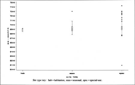
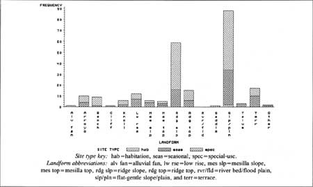
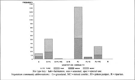
Each of the three habitation sites is at a different elevation, ranging from 6,840 to 6,920 ft (2,085 to 2,109 m) (Figure 6.11). There are more habitations than listed in Chapters 5 and 7 for this period because one Euro-American site is included in our analysis. Two of the sites are on a flat-gentle slope/plain and Pecos Pueblo is on the mesilla top (Figure 6.12). Habitations are either in grassland or grassland/piñon-juniper woodland vegetation (Figure 6.13).
|
| Figure 6.11. Box plot of elevation (in feet) by site type for Period 4 (A.D. 1450-1575). |
|
| Figure 6.12. Frequencies of each site type by landform types in Period 4 (A.D. 1450-1575). |
|
| Figure 6.13. Frequencies of each site type by vegetation community for Period 4 (A.D. 1450-1575). |
The elevation range of seasonal sites (n=89) is 6,780-7,300 ft (2,067-2,225 m), the same as Period 3 (A.D. 1325-1450); however, the distribution within that range changes as the percentage of sites above 7,000 ft (2,134 m) decreases (Figure 6.11). Seasonal sites are associated with 13 different landforms, although a flat-gentle slope/plain is the most common (Figure 6.12). Seasonal sites occur in a variety of vegetation communities, although three-quarters of them are in piñon-juniper woodland and grassland/piñon-juniper woodland (Figure 6.13).
Special-use sites (n=143) cover roughly the same elevation range as in Period 3 (A.D. 1325-1450), 6,750-7,420 ft (2,057-2,262 m) (Figure 6.11). There are thirteen different landforms represented in the locations of special-use sites; however, only two—flat-gentle slope/plain and ridge slope—are common (Figure 6.12). The percentage of special-use sites in piñon-juniper woodland and grassland/piñon-juniper woodland decreases slightly from the previous period. The percentage of sites in grassland increases slightly over Period 3, while it remains the same in piñon-juniper woodland/mixed conifer forest (Figure 6.13).
Period 5 (A.D. 1575-1700)
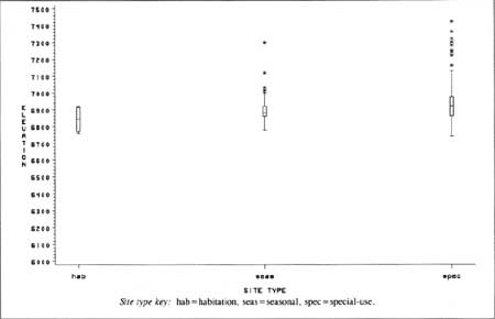
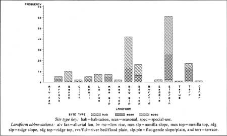
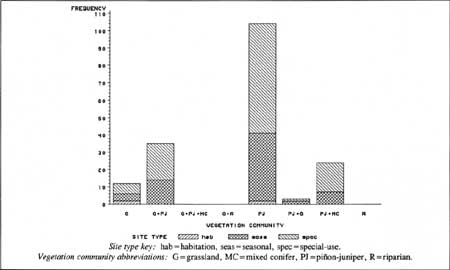
Habitations (n=4) in Period 5 (A.D. 1575-1700) occur between 6,760 and 6,920 ft (2,060 and 2,109 m) (Figure 6.14). Again, there are more habitations than listed in Chapters 5 and 7 for this period because two Euro-American sites are included in our analysis. There is a shift down in the lowest elevation, 6,760 ft (2,060 m), compared to the low of 6,840 ft (2,085 m) in Period 4 (A.D. 1450-1575). There is some variability in the landforms occupied—two sites are on a flat-gentle slope/plain, one is on the mesilla top, and one is on a terrace (Figure 6.15). The four habitations are in grassland and piñon-juniper woodland vegetation (Figure 6.16).
|
| Figure 6.14. Box plot of elevation (in feet) by site type for Period 5 (A.D. 1575-1700). |
|
| Figure 6.15. Frequencies of each site type by landform types in Period 5 (A.D. 1575-1700). |
|
| Figure 6.16. Frequencies of each site type by vegetation community for Period 5 (A.D. 1575-1700). |
Seasonal sites (n=66) are in a wide range of elevations, from 6,780 to 7,300 ft (2,067-2,225 m), although the majority is below 6,900 ft (2,103 m) (Figure 6.14). Seasonal sites occupy 11 different landforms, with a flat-gentle slope/plain the most common (Figure 6.15). More than 80 percent of seasonal sites are in piñon-juniper woodland and grassland/piñon-juniper woodland (Figure 6.16).
Special-use sites (n=108) range from 6,740 to 7,420 ft (2,054 to 2,262 m) in elevation, although more than 50 percent are below 6,900 ft (2,103 m) (Figure 6.14). Thirteen different landforms provide locations for special-use sites. The most common are a flat-gentle slope/plain and ridge slope (Figure 6.15). The percentage of special-use sites in the different vegetation communities is only slightly different than Period 4 (A.D. 1450-1575)—over three-quarters of the sites are in piñon-juniper woodland and grassland/piñon-juniper woodland (Figure 6.16).
Habitation Site Locations through Time
The elevation distribution of habitation sites changes slightly through time. There is one habitation site at 7,280 ft (2,219 m) in Periods 2 (A.D. 1200-1325) and 3 (A.D. 1325-1450) (Arrowhead, PECO 710, LA 251), but most are below 7,000 ft (2,134 m). Period 3 has the most habitation sites (n=10), and except for two outliers at 6,770 and 7,280 ft (2,063 and 2,219 m), the others are found within an 80-ft range. Spielmann (1991b) and Snow (1991) discuss the implications of short growing seasons and the difficulties of producing a successful harvest of mature, modern corn in the higher elevations of Pecos and New Mexico in general. Most Pecos habitations are above 6,600 ft (2,012 m), the level Snow (1991) identifies as too high, suggesting that agriculture was difficult at Pecos. As Snow (1991) notes, green corn can be harvested during a short growing season, but this would not provide any seed corn.
A flat-gentle slope/plain is the most common landform in each period. Because of the small number of habitations in each period, it is probably not very meaningful to draw conclusions from the distributions. There do not seem to be other locational trends except the persistent occupation of the mesilla beginning in Period 3 (A.D. 1325-1450). The greatest variety of landforms associated with habitations is in Period 3, the period with the most habitations.
Modern vegetation communities at Pecos are a product of heavy, relatively recent manipulation of the environment (Sivinski 1995; see Chapter 5). Therefore, their usefulness for interpreting prehistoric or early historic site locations is questionable. Piñon-juniper woodland and grassland/piñon-juniper woodland are the predominant vegetation communities associated with habitation sites in Periods 2 (A.D. 1200-1325) and 3 (A.D. 1325-1450). Period 4 (A.D. 1450-1575) habitations are in grassland and grassland/piñon-juniper woodland, and Period 5 (A.D. 1575-1700) sites are evenly split between grassland and piñon-juniper woodland vegetation communities. Even though we can identify trends and change through time, we are not sure how modern vegetation relates to prehistoric vegetation so it is difficult to relate settlement decisions to the distribution of modern vegetation communities.
Seasonal Site Locations through Time
Seasonal sites in Period 2 (A.D. 1200-1325) cover the smallest elevation range; this range expands during Period 3 (A.D. 1325-1450), along with an increase in the number of sites. When the number of sites decreases in Periods 4 (A.D. 1450-1575) and 5 (A.D. 1575-1700), the elevation range does not shrink. Like habitation sites, seasonal sites, most of which we assume are agricultural field houses, are found at elevations presumably too high for successful agriculture. Elevation range is not the most diverse in Period 2 (A.D. 1200-1325), the driest period, nor is it the least diverse in the wetter periods, contrary to what we expected based on the PDSI.
There is some variability in the types of landforms used through time, although a flat-gentle slope/plain is the most common in each period. Ridge slope and terrace are also fairly common beginning in Period 3 (A.D. 1325-1450). If the seasonal sites in Periods 2-5 (A.D. 1200-1700) are field houses, it is obvious that a great deal of effort was invested in distributing them over a diversity of landscapes. As the number of seasonal sites increases in Period 3, so do the number of landforms used. This variety is maintained in Periods 4 (A.D. 1450-1575) and 5 (A.D. 1575-1700) despite decreasing numbers of sites. Apparently, locational diversity was a goal in all periods, which does not conform to our expectations based on the PDSI dryness index. We expected diversity to decrease after Period 3 because there are fewer sites and potential agricultural productivity increases.
Piñon-juniper woodland and grassland/piñon-juniper woodland are the two most common vegetation communities at seasonal sites in all periods. Seasonal sites in Period 3 (A.D. 1325-1450) occur in the greatest variety of vegetation communities (n=6), followed by Periods 2 (A.D. 1200-1325) and 4 (A.D. 1450-1575), with five communities represented in each. These distributions may have little meaning for interpreting site distributions because prehistoric vegetation probably consisted of more grassland and less piñon-juniper woodland (Sivinski 1995).
Special-use Site Locations through Time
The elevation range represented in special-use site locations is smaller in Period 2 (A.D. 1200-1325) than Periods 3-5 (A.D. 1325-1700). Once the range expands in Period 3 (A.D. 1325-1450), it does not contract, except for the disappearance of one very low elevation site in Period 5 (A.D. 1575-1700), even when site numbers decrease. The range suggests that the population always exploited a variety of resources, which is contrary to an expected decline in diversity based on the PDSI.
Although the most common landforms associated with special-use sites through time are a flat-gentle slope/plain and ridge slope, there is great diversity of landforms in Periods 3-5 (A.D. 1325-1700). Ridge slopes represent a much higher percentage of the locations in Periods 4 (A.D. 1450-1575) and 5 (A.D. 1575-1700) than in previous periods. The continued use of a diverse number of landforms in periods with fewer sites points to the amount of effort invested in maintaining variety, even when the PDSI indicates more favorable conditions for agriculture.
Piñon-juniper woodland and grassland are the most common vegetation communities at special-use sites in Periods 2-5 (A.D. 1200-1700). Although special-use sites outnumber seasonal sites in all periods, they are associated with fewer vegetation communities (n=4 for each period) than seasonal sites in Periods 2-4 (A.D. 1200-1575).
Overall it appears that habitation sites stay in much the same elevations and landforms through time. Period 3 (A.D. 1325-1450) sees a great expansion in the diversity of elevation and landforms for both seasonal and special-use sites. Contrary to expectations derived from the characterization of climate change, this diversity is maintained in subsequent periods.
Social Influences on Site Location
In an effort to examine potential social and economic influences on activity locations, this portion of the chapter characterizes the spatial association of sites within each time period. The method used will compare the distribution of the observed distances between sites to those expected for a simulated random distribution of sites. The nearest-neighbor distance (NND) between sites of specific types is measured, and statistical comparisons use the median NND (mNND) for each assemblage of sites.
While the other sections of this chapter seek to better understand the effects of the natural environment on decisions about site and activity location, this analysis seeks to determine whether the placement of contemporaneous sites is to some degree influenced by the locations of other sites. Although this discussion is primarily descriptive (in terms of the characterization of the relationship between sites), there are several hypotheses related to the spatial distribution of sites relative to each other that will be examined. First, in reference to special-use and seasonal sites, the following hypotheses are evaluated:
Hypotheses 1-3: Nearest-neighbor distances for special-use and seasonal sites, both within each site type (Hypothesis 1: between special-use sites, Hypothesis 2: between seasonal sites) and between the two site types (Hypothesis 3: between special-use and seasonal sites) should reflect more clustering as population density increases. This is expected as a result of the increasing intensification of landscape use through the pursuit of agricultural (seasonal sites) and wild resource procurement (special-use sites) activities in previously unutilized intermediate locations.
Hypotheses 4-5: It is expected that the large population concentration at Pecos Pueblo will have a negative impact on local resources, depleting them over time. Nearest neighbor values between special-use and habitation sites (Hypothesis 4) and between seasonal sites and habitation sites (Hypothesis 5) are expected to reflect greater dispersion as resource extraction activities must take place farther away from the large pueblo.
In reference to habitation sites, the following hypothesis is evaluated:
Hypothesis 6: As population density increases, a pattern of increased dispersion among habitations is expected because it becomes necessary to clearly define territories to minimize competition and conflict for resources.
It is important to note that this analysis addresses only one set of factors—those that relate to the relative positioning of sites to each other—out of many that might influence site location.
Traditional Spatial Analysis Methods
There are several methods to evaluate spatial patterning of sites or, more generally, the analysis of point patterns in data (Bailey and Gatrell 1995:75-139; Ripley 1981:102-190, 1991:22-48). In most cases, archeological site distributions are compared to those expected if site patterning were random. This type of analysis is often presented in reference to a continuum between clustered points and evenly dispersed points, with the corresponding patterns then interpreted in behavioral terms. While there are a variety of approaches to examine site-to-site patterning, the two most frequently employed in archeology are quadrat analysis and nearest-neighbor analysis (Hodder and Orton 1976).
Quadrat Analysis
Quadrat analysis subdivides an area into units of equal size. Within each, the frequency of events of interest (e.g., archeological sites) is counted. Examination of the distribution of observed frequencies within quadrats allows us to determine whether that distribution differs from a random one. Specifically, the ratio of the variance to the mean frequency is used to determine whether the observed patterning is more closely associated with clustering (high ratio values) or dispersion (low ratio values). A ratio of 1 is interpreted as random spacing, a ratio greater than 1 suggests clustering, and a ratio less than 1 indicates dispersion. This numeric interpretation is based upon the expected behavior of a Poisson process in which rare events are randomly distributed through space (or time).
Problems with quadrat analysis commonly arise in archeological research. In particular, small mean frequencies within each cell may yield erratic results. This situation is analogous to a chi-square analysis in which the expected values for a large number of cells are less than 5. Related to this issue is the influence that quadrat size and shape have on the results. One obvious impact is that with small quadrats, there will be fewer sites, which may yield mean frequencies that are too small to be dependable. Other important effects of quadrat size result from the relationship between the size of quadrats used and the spatial patterning of the phenomena under analysis. For example, if site clusters are larger than the size of the quadrats, this tends to lessen the "signal" for clustering because the clusters will overlap several quadrats, decreasing the variance and mean frequencies (though not in proportion to each other). On the other hand, if the quadrats are as large as the spacing between clusters of sites, the distribution will appear more random than with smaller quadrats. Quadrat shape has also been noted to influence the values obtained in the analysis, again highlighting the impact of analytic decisions on the interpretation of the results (Bailey and Gatrell 1995:84, 96-98). Nearest-neighbor analyses have been proposed to circumvent some of these problems.
Nearest-Neighbor Analysis
Nearest-neighbor analyses have the potential to mitigate some of the problems noted for quadrat-based analyses, particularly the effects of quadrat size and shape. Nearest-neighbor analysis measures the distance between one location and the nearest location of interest (Bailey and Gatrell 1995:89-90). For example, a nearest-neighbor analysis of the relationships between habitation sites measures the distance from one habitation to the next nearest habitation site. This process is repeated for each habitation site in the area of consideration, with the resulting distances providing an estimate of the average (or median) nearest-neighbor distance for all sites of that type. This value can then be compared to the expected nearest-neighbor distance to determine whether the observed value is significantly different. In general, the expected nearest-neighbor distance is determined from the ratio of the size of the area to the number of sites in the area. If the observed nearest-neighbor distance is greater than the expected value, the conclusion is that the sites are more uniformly distributed than expected from a random distribution. On the other hand, if the observed distance is less than the expected value, clustering is inferred.
Traditional nearest-neighbor analyses also have problems, particularly edge effects and decreased utility when site frequencies are small. Edge effects refer to bias introduced into the calculated nearest-neighbor distances through the influence of sites located near the boundary of the analysis area. These effects result from the fact that, in many cases, the analysis boundaries artificially demarcate space, potentially eliminating sites that may be the nearest neighbors but are outside the area of consideration. This phenomenon has the potential to artificially increase the estimated nearest-neighbor distance. Often, establishing a buffer zone within the outer edge of an analysis area within which nearest-neighbor distances will not be calculated mitigates edge effects. An alternative approach is to "wrap-around" from one side of the analysis area to the opposite side, essentially creating a three-dimensional surface over which distances are calculated. One significant drawback to this approach is that it requires rectangular analysis areas to facilitate the "wrap" (Bailey and Gatrell 1995; Ripley 1981). Finally, in order to use tests of significance in evaluating deviations from randomness, the number of locations used in the analysis should be greater than 50 (Hodder and Orton 1976). This requirement often limits the use of nearest-neighbor analyses in some archeological contexts.
Conclusions Regarding Traditional Spatial Analysis Methods
The preceding discussion outlined the general characteristics of two methods commonly used to examine the spatial relationships among sites. One characteristic that both quadrat and nearest-neighbor analysis share is the fact that both are based upon an assumed underlying distribution, the Poisson for quadrat analysis and the normal distribution for nearest-neighbor analysis. The assumed distributional characteristics of Poisson or normal distributions contribute to some of the problems noted above, particularly in cases where sample sizes are small, or values are biased because of problems such as edge effects. A simulation-based approach was utilized in this analysis to avoid or mitigate some of the problems noted above for nearest-neighbor analyses.
Simulation-based Nearest-Neighbor Analysis
We have made an effort to overcome some of the problems associated with traditional nearest neighbor analyses by comparing observed nearest-neighbor distances to expected distances derived from simulations. Significance tests were performed by comparing the observed NND to the NND values for the simulated assemblages of sites. The major advantages of this simulation approach are the distributional independence of the significance tests and the mitigation of edge effects by generating expected values that also reflect edge effects, therefore controlling for potential bias in the observed data sets when compared to theoretical data.
Simulation Analysis Methods
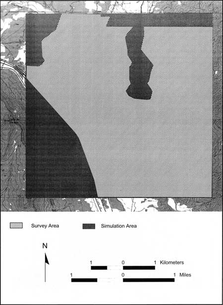
The general procedure employed in the simulations was one in which randomly distributed points were generated within a rectangular region whose dimensions were defined using the northern-, southern-, eastern-, and westernmost site locations in the survey area (regardless of period) as the source for the coordinates for the northern, southern, eastern, and western boundaries for the simulation rectangle (Figure 6.17). This results in a simulation region somewhat larger than the survey area. The number of random points generated in each simulation corresponds to the number of sites for the period under consideration (Table 6.2). Random points were generated 500 times for each comparison.
| Table 6.2. Number of sites simulated for each period. | |||
| Site Type | |||
| Period | Special-Use | Habitation | Seasonal |
| 0 (pre A.D. 1075) | — | — | 3 |
| l (A.D. 1075-1200) | l | — | l |
| 2 (A.D. 1200-1325) | 56 | 6 | 39 |
| 3 (A.D. 1325-1450) | 188 | 10 | 104 |
| 4 (A.D. 1450-1575) | 143 | 3 | 89 |
| 5 (A.D. 1575-1700) | 107 | 4 | 66 |
| 6 (post A.D. 1700) | 35 | 3 | 20 |
|
| Figure 6.17. Simulation region in comparison to survey area. (click on image for an enlargement in a new window) |
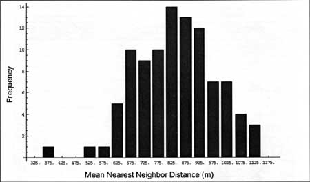
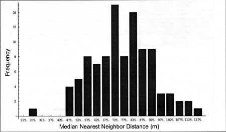
For example, in the analysis of the distances between special-use sites and habitation sites in Period 2 (A.D. 1200-1325), six habitation sites and 56 special-use sites were identified. In the simulation of relationships between these sites, 56 random special-use site locations and six random habitation site locations were generated. Nearest-neighbor distances were then determined for each of five hundred sets of random points generated for each simulation, yielding frequency distributions of mean and median NND values (Figures 6.18 and 6.19). The frequency distributions of these means and medians were then used to calculate significance values to assess the direction and magnitude of the deviation of the observed NNDs from the expected simulated random distribution. The simulated random distribution is thus used in lieu of the Poisson or normal distributions underlying traditional spatial analyses.
|
| Figure 6.18. Frequency distribution of mean NND between habitations in Period 3 (A.D. 1325-1450). |
|
| Figure 6.19. Frequency distribution of medium NND between habitations in Period 3 (A.D. 1325-1450). |
The magnitude and direction of deviations from randomness are determined by calculating the proportion of the simulated means or medians that are less than the observed value. If a large or small proportion—97.5 percent or 2.5 percent for a significance level (a) of .05—of the simulated mean or median distances is less than the observed mean or median distance, one can conclude that the observed values deviate significantly from random. If a large proportion of the simulated distances are less than that observed, dispersion is indicated. Conversely, if a small proportion of the simulated distances are less than the observed, clustering is indicated. In those instances where a nonsignificant proportion of the simulated mean or median distances differ from the observed proportion, the null hypothesis (Ho) of random patterning (or independence) cannot be rejected.
The following nearest-neighbor simulations were run in each period:
- special-use to special-use (spec-spec in tables and figures),
- special-use to habitation (spec-hab),
- special-use to seasonal (spec-seas),
- habitation to habitation (hab-hab),
- habitation to seasonal (hab-seas), and
- seasonal to seasonal (seas-seas).
In some cases there were no sites of a given type in a particular period, so that out of a total of 42 possible simulations, 34 actually yielded results.
The absolute number of sites observed in a particular period plays a significant role in determining the nearest-neighbor distances that are obtained both through simulation and observation. In cases where the number of sites is large, we would expect nearest-neighbor distances to be lower purely as a function of packing more sites into a nonexpanding spatial area. Since the simulations take into account the number of sites of each type in the comparison, the resulting significance tests reflect deviations from a random distribution that uses the same number of sites, thus taking into account fluctuations in distance that are a function of increasing or decreasing site frequencies.
Results of Simulated Nearest Neighbor Analysis
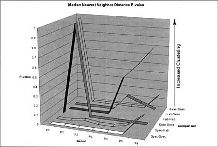
The results presented below are organized by comparison with consideration of both significance of values obtained within each period, and diachronic variation in the observed NNDs. The results are summarized in Table 6.3 and Figure 6.20 and discussed in the following sections. While mean NNDs are presented for each analysis, the following discussion utilizes the median (referred to hereafter as mNND) because some markedly asymmetric distributions exist in which the mean is not a reasonable measure of central tendency in the observed data. This disparity is illustrated by the dramatic change in p values for some of the simulations presented in Table 6.3—differences ranging from one extreme to another (i.e., clustering to dispersion as in Period 2 (A.D. 1200-1325) for Habitation-Seasonal (Table 6.31)—depending on whether the p value is calculated from the distribution of mean or median simulated values and compared to the corresponding observed values.
|
| Figure 6.20. Median NND p value by period and site type comparison. |
| Table 6.3. Nearest-Neighbor simulation results. | |||||
| Comparisona | Period | Mean NND (m) | p value Mean NNDb |
Median NND (m) | p value Median NNDb |
| Spec-Spec | 0 | — | — | — | — |
| 1 | — | — | — | — | |
| 2 | 247.22 | .0000 | 144.03 | .0000 | |
| 3 | 137.16 | .0000 | 100.49 | .0000 | |
| 4 | 163.44 | .0000 | 104.64 | .0000 | |
| 5 | 216.00 | .0000 | 195.26 | .0000 | |
| 6 | 455.70 | .4460 | 379.36 | .1760 | |
| Spec-Hab | 0 | — | — | — | — |
| 1 | — | — | — | — | |
| 2 | 1086.69 | .0000 | 1075.83 | .0220 | |
| 3 | 809.44 | .0000 | 696.84 | .0000 | |
| 4 | 1212.19 | .0000 | 1096.99 | .0000 | |
| 5 | 1248.05 | .0720 | 1143.02 | .0360 | |
| 6 | 1371.00 | .1180 | 1291.16 | .1520 | |
| Spec-Seas | 0 | — | — | — | — |
| 1 | 5358.25 | 1.0000 | 5358.25 | 1.0000 | |
| 2 | 424.82 | .5660 | 263.58 | .0020 | |
| 3 | 254.11 | .1960 | 197.27 | .0000 | |
| 4 | 313.11 | .5900 | 216.83 | .0000 | |
| 5 | 376.47 | .8220 | 237.35 | .0000 | |
| 6 | 568.15 | .1580 | 413.49 | .0020 | |
| Hab-Hab | 0 | — | — | — | — |
| 1 | — | — | — | — | |
| 2 | 1501.06 | .8120 | 308.85 | .0000 | |
| 3 | 1084.47 | .6000 | 484.88 | .0040 | |
| 4 | 840.13 | .9760 | 387.74 | .4200 | |
| 5 | 829.25 | .5140 | 829.27 | .5720 | |
| 6 | 1916.83 | .9880 | 1270.81 | .7580 | |
| Hab-Seas | 0 | — | — | — | — |
| 1 | — | — | — | — | |
| 2 | 909.94 | .9840 | 151.06 | .0020 | |
| 3 | 564.04 | 1.0000 | 153.12 | .0020 | |
| 4 | 151.43 | .1100 | 147.64 | .1700 | |
| 5 | 205.80 | .1180 | 181.01 | .1100 | |
| 6 | 235.00 | .0260 | 214.66 | .0560 | |
| Seas-Seas | 0 | 126.09 | .9880 | 112.97 | .9680 |
| 1 | — | — | — | — | |
| 2 | 212.25 | .0000 | 160.80 | .0000 | |
| 3 | 158.17 | .0000 | 108.07 | .0000 | |
| 4 | 191.11 | .0000 | 159.35 | .0000 | |
| 5 | 234.26 | .0020 | 198.90 | .0000 | |
| 6 | 490.95 | .4400 | 389.97 | .1600 | |
aSpec = Special Use, Hab = Habitation, Seas = Seasonal bProportion of simulated values that are less than that observed. P values <0.025 or >0.975 would be considered significant at the a=0.05 level and are shaded. | |||||
Comparison of Special-Use to Special—Use Sites
Special-use sites are significantly clustered (mNND p value < 0.025) for all periods except Period 6 (post A.D. 1700). This is not surprising since these sites probably represent resource gathering and processing locations that would be in close proximity to the materials being gathered or processed. Because resources across the landscape tend to be spatially correlated (i.e., there may be several productive areas near each other, or large productive areas may exist that are utilized repeatedly or contemporaneously), clustering of sites related to these resources is expected. The fact that there is no significant deviation from randomness in Period 6 may be related to the substantial decrease in the number of special-use sites, yielding an overall low density of sites on the landscape. The decrease in site density may be associated with a more spatially extensive wild resource utilization strategy that was not closely tied to the clustering of productive areas. It may also represent disuse of much of the study area due to the threats from Comanche raiding that were prevalent at Pecos during the eighteenth century.
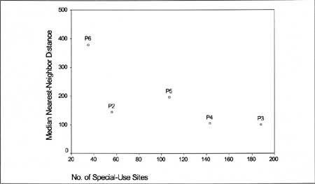
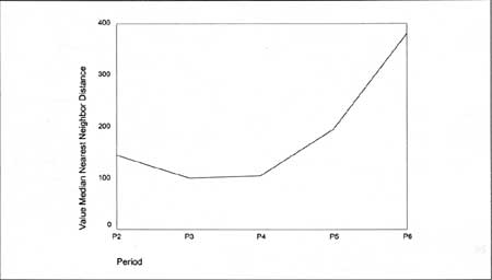
The plots of mNND against the number of sites for each period (Figure 6.21), the mNND by period (Figure 6.22), and the mNND p values by period (Figure 6.20) illustrate the temporal trends in these relationships. Specifically, they demonstrate the strong negative correlation between the mNND and the number of sites (Figure 6.21). As the number of sites increases, the mNND decreases, and the mNND p values remain consistently significant in their indication of clustering. This trend supports Hypothesis 1 (outlined at the beginning of this section), insofar as this hypothesis predicts a decrease in mNND values among special-use sites as population density increases. When plotted by period (Figure 6.22), the low point in the curve of mNND values occurs in Period 3 (A.D. 1325-1450), the peak in local population. This relationship reinforces the interpretation that the intensity of patch utilization is driving the significant clustering, with the special-use site densities in Period 6 (post A.D. 1700) perhaps crossing a threshold where individual resource patches are occupied by one or fewer special-use sites.
|
| Figure 6.21. Plot of observed median NND for special-use sites vs. the number of special-use sites in each period. |
|
| Figure 6.22. Median observed N?ND between special-use sites by period. |
Comparison of Special-Use to Habitation Sites
Habitation and special-use sites are significantly clustered in Periods 2 (A.D. 1200-1325), 3 (A.D. 1325-1450), and 4 (A.D. 1450-1575), while there is no significant clustering or dispersion in Periods 5 (A.D. 1575-1700) and 6 (post A.D. 1700). This result is consistent with a conclusion that special-use sites, while being associated with patches of resources (see above and localized plant productivity analysis in later section), are also selected based upon proximity to habitation sites. This supports Hypothesis 4 for greater dispersion of habitation and special-use sites with increasing population density. It also is consistent with the common sense conclusion that populations will first tend to utilize resources close to their place of residence before taking advantage of more distant resources.
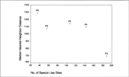
Another interesting trend in the relationship between special-use and habitation sites is the nonlinear relationship between the number of special-use sites and the mNND between special-use and habitation sites (Figure 6.23). The plateau in the middle of the distribution, particularly for Periods 4 (A.D. 1450-1575) and 5 (A.D. 1575-1700), suggests that distances between special-use and habitation sites are not decreasing with increasing frequency of special-use sites, as would be expected due to the simple process of packing additional sites into a limited area. This may be related to an increasing need to utilize resources more distant from large aggregated habitation sites like Pecos Pueblo. This result again is consistent with the expectation outlined in Hypothesis 4 at the beginning of this section of the chapter—that as population grows at specific locations, local resources may be inadequate to meet the requirements of the aggregated population. The fact that Periods 5 and 6 (post A.D. 1700) also showed no significant clustering between special-use and habitation sites (Table 6.3; Figure 6.20) further reinforces this argument. Specifically, while habitation and special-use sites are clustered in Periods 2-4 (A.D. 1200-1575) suggesting a consistent utilization of local resources, it is possible that localized resource inadequacy or depletion led aggregated populations in Periods 5 and 6 to exploit resources more distant from their settlements. An alternative explanation for this pattern is that the patchiness of resources prevents the establishment of sites at intermediate locations, leading to a bottom limit below which mNND values cannot exist. While these suggestions can not be evaluated with the available survey data, they present interesting questions for further study.
|
| Figure 6.23. Plot of observed median NND between special-use and habitation sites vs. the number of special-use sites for each period. |
Overall, the trends observed in the relationship between special-use and habitation sites are consistent with a generalized pattern of localized resource use, with increasingly distant resources exploited as local resources become depleted. This conclusion is supported through both the nonlinear trend in the relationship between the number of special-use sites and the observed mNND, and the transition from a clustered to a random pattern of association between these site types through time.
Comparison of Special-Use to Seasonal Sites
Excluding Period 1 from discussion (pre A.D. 1075) because of an insufficient sample (n=1 for each site type), special-use and seasonal sites are significantly clustered in Periods 2, 3, 4, 5, and 6 (A.D. 1200-1700+) (Table 6.3; Figure 6.20). Environmental factors probably play an important role in this relationship. Specifically, the environmental conditions conducive to agricultural production are also conducive to wild plant production, leading to co-occurrence of special-use and seasonal sites.
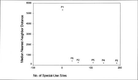
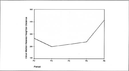
There seems to be a relative insensitivity of the mNND to the number of special-use sites in a given period (Figure 6.24). It is possible that land use within the 200-400 m (656-1,312 ft) distances indicated by the mNNDs in Periods 2-5 (A. D. 1200-1700) (Figure 6.25) occurs at a relatively constant rate and that additional resource acquisition (through the complementary activities of agriculture and wild resource acquisition) is achieved through spatial expansion as opposed to localized intensification. If this were not the case, one would expect to find a negative correlation between the number of sites and the mNND, because localized intensification would have the effect of reducing the mNND for periods with greater intensification.
|
| Figure 6.24. Plot of observed median NND between special-use and season sites vs. the number of special-use sites in each period. |
|
| Figure 6.25. Median observed NND between special-use and seasonal sites by period. |
This conclusion fails to support Hypothesis 3 (outlined above) that NND values between special-use and seasonal sites should decrease as population density increases. This conclusion is also inconsistent with the results of the comparison among special-use sites (Hypothesis 1), in which the mNND decreased as the number of special-use sites increased. This inconsistency may be the result of a differential labor investment in components at special-use as opposed to seasonal sites. Because of the investment of labor in building architectural features and preparing fields at seasonal sites, they may be more likely to be reoccupied than special-use sites, therefore reducing the number of sequentially occupied seasonal sites when compared to special-use sites. This pattern of differential reoccupation may lead to the different conclusions outlined above. When considered by themselves, special-use sites have a lower probability of reoccupation, therefore increasing the likelihood for nearby, sequentially occupied sites, leading to an interpretation of intensification where sequential occupation may be a valid alternative explanation.
Overall, the relationship between special use and seasonal sites suggests clustering and a constant NND for each period except Period 1 (pre A.D. 1075). In contrast with Hypothesis 3 (outlined above), these results are consistent with an interpretation of relatively constant intensity of land use, independent of population. One by-product of this inference is that as additional resources were required for a growing population, those resources may have been obtained through a more spatially extensive—as opposed to intensive—acquisition region, or through an increase in trade, although these suggested explanations cannot be evaluated with the current survey data.
Comparison of Habitation to Habitation Sites
Habitation sites were clustered in Periods 2 (A.D. 1200-1325) and 3 (A.D. 1325-1450). During Periods 4-6 (A.D. 1450-1700+) there are no significant deviations from randomness (Table 6.3; Figure 6.20). Specifically, the mNNDs for Periods 2 and 3 are significantly smaller than those obtained through simulation. In contrast, the mNNDs for Periods 4-6 (A.D. 1450-1700+) are within the range of variation obtained in the simulation. These differences define two distinct patterns, one temporal and the other spatial.
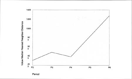
The fact that there is significant clustering—and relatively small mNNDs (Figure 6.26)—in only the earlier periods suggests that prior to the development of Pecos Pueblo there was little competition for resources among communities. If localized resources were inadequate to support the habitation sites extant during Periods 2 (A.D. 1200-1325) and 3 (A.D. 1325-1450), the sites would not be clustered. This interpretation is reinforced by the subsequent dispersal of habitation sites into a nonclustered—but not evenly dispersed—distribution. The concentration of population at Pecos Pueblo may have had a substantial impact on local resources, necessitating the location of other habitation sites farther away from Pecos.
|
| Figure 6.26. Median observed NND between habitation sites by period. |
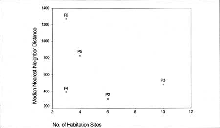
There was a qualitative change in the spatial relationships between habitation sites following the appearance of Pecos Pueblo, with these changes providing strong support for Hypothesis 6 (outlined above). Specifically, there was a relatively constant mNND for habitation sites in Periods 2-4 (A.D. 1200-1575) (Figure 6.26), but mNND values increase substantially in Periods 5 (A.D. 1575-1700) and 6 (post A.D. 1700) while the number of habitation sites is small—four in Period 5, three in Period 6 (Figure 6.27) (these site counts do not agree with Table 7.1 because the nearest-neighbor dataset includes Euro-American sites).
|
| Figure 6.27. Plot of observed median NND between habitations vs. the number of habitations in each period. |
The expectation that increasing population density would lead to increasing dispersion of habitations (Hypothesis 6), is supported by the results of the NND analysis. There is indeed evidence that habitations become more dispersed as population increases through Period 3 (A.D. 1325-1450), and this trend toward dispersion continues after Period 3 (Figure 6.20), accompanying continuing aggregation and despite the decline of population in the Pecos area (see Figure 7.1).
These changes in the spatial organization of habitation sites suggest that there were fundamental shifts in how individual communities related to each other and to the land from which they derived their living. With increased local impacts resulting from population aggregation, it became necessary to live farther and farther from other habitations in order for local populations to support themselves and avoid conflicts over resources.
Comparison of Habitation to Seasonal Sites
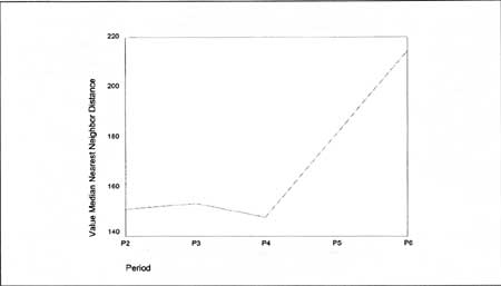
Like the trends observed among habitation sites, habitation and seasonal sites are clustered in Periods 2 (A.D. 1200-1325) and 3 (A.D. 1325-1450), and there are no significant deviations from randomness in Periods 4, 5, and 6 (A.D. 1450-1700+). Although the mNNDs are substantially lower than those between habitation sites (compare Figure 6.26 to Figure 6.28), the temporal and spatial patterning are remarkably similar.
As was found among habitation sites, there is a trend away from clustering after Period 3 (A. D. 1325-1450) (Figure 6.28). This finding supports Hypothesis 5, outlined above, expecting greater dispersion between habitation and seasonal sites with increasing aggregation. As habitation locations become more stable with substantial investments in architectural features, new agricultural sites are established farther and farther from the habitations.
|
| Figure 6.28. Median observed NND between habitations and seasonal sites by period. |
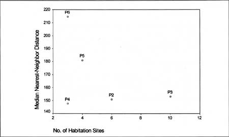
The spatial patterning between habitations and seasonal sites is also strikingly similar to that observed between habitation sites. Specifically, the mNNDs between habitation and seasonal sites appear independent of the number of habitations (albeit low) throughout all periods (Figure 6.29). This may also be related to the increased dispersal of agricultural fields through time, independent of the number of habitation sites.
|
| Figure 6.29. Plot of observed median NND between habitations and seasonal sites vs. the number of habitations in each period. |
Comparison of Seasonal to Seasonal Sites
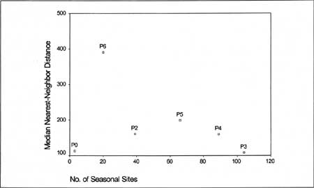
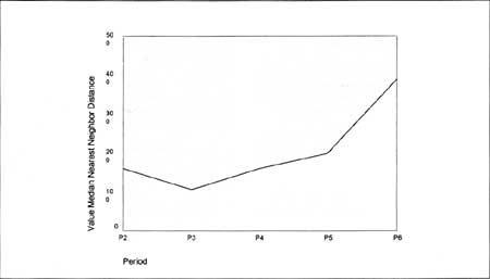
Like the relationships among special-use sites, the relationships among seasonal sites is characterized by significant clustering for Periods 2, 3, 4, and 5 (A.D. 1200-1700), with decreasing mNND values associated with greater numbers of seasonal sites (Figure 6.30), and increasing mNND values starting in Period 3 (A.D. 1325-1450) (Figure 6.31). These results support Hypothesis 2 (outlined above), and the expectation that NND values among seasonal sites will decrease with increasing population density. These trends are consistent with the pattern of environmental productivity (as discussed in the analysis of the relationship between special-use and seasonal sites) influencing the concentration of agricultural fields within more productive subregions, leading to clustering of seasonal sites.
|
| Figure 6.30. Plot of observed median NND between seasonal sites vs. the number of seasonal sites in each period. |
|
| Figure 6.31. Median observed NND between seasonal sites by period. |
Only about one-third of the relationships examined in the nearest-neighbor analysis are something other than clustered. With seasonal and special-use sites, the high degree of clustering both within and between these site types supports the conclusion that these locations were largely determined by resource availability, with those resources closest to the habitation site being used first. Nonhabitation sites were moved farther away from habitations through time, suggesting that localized resource depletion may have played a role in the relationship between habitation and resource procurement locations.
Special-use and seasonal sites are clustered in every period, and are the only comparison to show that consistency through time. It is likely that the same factors favoring agriculture also favor wild plant production so that resource locations encouraged multiple strategies in the same area.
In reference to the hypotheses outlined at the beginning of this section, the following comments can be made:
Hypothesis 1, that increasing population densities would be associated with decreasing NND values among special-use sites, received strong support in this analysis.
Hypothesis 2, that increasing population densities would be associated with decreasing NND values between seasonal sites, also received strong support in this analysis.
Hypothesis 3, that increasing population densities would be associated with decreasing NND values between special-use and seasonal sites, received no significant support.
Hypothesis 4, that local resource depletion around Pecos Pueblo would increase NND values between special-use and habitation sites, received strong support in this analysis. The analysis also revealed that the NND values remained high even when the number of special-use sites increased.
Hypothesis 5, that local resource depletion would increase NND values between seasonal and habitation sites, received strong support in this analysis.
Hypothesis 6, that increasing population density would create increase NND values among habitation sites received strong support in this analysis.
Habitation sites are clustered in Periods 2 (A.D. 1200-1325) and 3 (A.D. 1325-1450), suggesting that resource competition between communities may not play a strong role in determining the spatial relationship between communities during these periods. Habitations in Periods 4-6 (A.D. 1450-1700+) are increasingly dispersed, with their relative distribution not significantly different from that expected for a random distribution of sites. Although this is not a case of even spacing between sites, a situation indicative of conflict, the move from clustered to random distributions and the greater distances between sites probably points to resource competition between habitation sites during the later periods of occupation. This result is consistent with the expectations associated with Hypothesis 6, that with the aggregation of population at Pecos Pueblo mNND values would increase as a result of necessary dispersion of habitation sites to locales outside the resource procurement zone surrounding Pecos. Specifically, the trend in habitation site dispersion (relative to other habitation sites) supports Hypothesis 6 through Period 4 (A.D. 1450-1575), but the continuing dispersion of sites through Periods 5 and 6 (A.D. 1575-1700+) is contrary to this expectation.
Overall, this analysis has provided a summary of the spatial relationships between the three major site types identified within the Pecos CRIS study area. While consideration of the relationships between sites only addresses one set of variables that influence the location of human activities on the landscape, when integrated with the results of other analyses in this chapter, it provides an important insight into how the cultural landscape at Pecos was formed.
Site Location and Localized Soil and Resource Productivity
As part of the analysis of environmental conditions influencing the selection of particular locations for different activities, this last section of the chapter summarizes the results of an analysis of the local plant productivity immediately proximate to site locations. As mentioned in the first part of the chapter, recent vegetation is not always representative of past conditions, especially in an area that has been so long affected by human use as the Upper Pecos Valley. Characterization of potential plant productivity of soils should more directly reflect the prehistoric setting, since the nature of soils is relatively immutable. Unlike the data taken from the site forms, this approach also uses information on areas that are not archeological sites, providing more detailed characterization of site placement.
This analysis considered each of the three functional site types separately, regardless of time period. The decision to combine sites from different periods was made for three reasons. First, it is assumed that the activities associated with each site type are relatively constant through time (i.e., agricultural activities at seasonal sites, wild resource collection and processing at special-use sites). Second, we assume that the general conditions represented by the plant productivity estimates from the Pecos Soil Survey (Soil and Water West 1996) are relatively constant through time. Third, subdividing the sites into discrete periods would reduce the number of sites in each analysis, yielding smaller sample sizes for each site type.
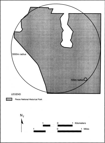
Overall, this analysis seeks to determine if there are significant relationships between the localized productive potential of soils for economic plant species and the locations of habitation, special-use, and seasonal sites. In contrast to traditional catchment analyses in which polygonal regions of more than 3 km (1.9 mi) in diameter are employed to examine the influence of regional resource availability on site location (e.g., Van West 1994, Varien 1999), this analysis employs relatively very small 100-m radius "catchments" to differentiate between the areas upon which sites are found and those where they are not found. This small "buffer" (used here as a more appropriate term than "catchment") size is better suited to the relatively small survey area for this project. As can be seen in Figure 6.32, larger catchment radii of sizes traditionally employed in catchment analysis would effectively eliminate the "nonsite" catchment component for the Pecos survey area. In the absence of comparable site and nonsite catchment areas, a standard catchment analysis is impossible. Furthermore, the use of small site buffer areas allows for more precise characterization of specific site location criteria than would large catchment areas.
|
| Figure 6.32. Comparison of 3-km radius catchment and 100-m radius buffer area. (click on image for an enlargement in a new window) |
Potential Plant Productivity of Soils
The recent soil survey of Pecos National Historical Park (Soil and Water West 1996) provides qualitative estimates of the potential productivity for different plant classes of the soil units mapped in the project area. The specific plant productivity potentials used in this analysis fall into two groups: those associated with food production or gathering and those that, while having potential food value, may also provide fuel wood. Within the food-related group, the following three classes of resources are considered: grain and seeds, grasses, and herbaceous plants. Within fuel woods, coniferous species and shrubs are considered.
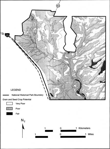
Productivity values assigned by the soil survey range from 0 (Very Poor) through 2 (Fair) to a maximum value of 4 (Very Good). These are best conceptualized as relative qualitative measures of productivity, where higher is more productive, rather than absolute, quantitative figures. Figure 6.33 illustrates the mapped grain and seed productivity potentials provided by the soil survey as an example. Similar mapped distributions exist for the other vegetation classes used in the analysis. In Figure 6.33 the western boundary of the soil survey does not coincide with the current park boundary because at the time of the soil survey the park boundary did not extend to the interstate.
|
| Figure 6.33. Grain and seed productivity for Pecos National Historical Park based on soil survey data. (click on image for an enlargement in a new window) |
The particular economic plant species (Soil and Water West 1996:Table 4, 72-73), their potential uses (Dunmire and Tierney 1997:270-283), and likely classification within the categories defined by Soil and Water West (1996) are shown in Table 6.4. The economic categories in Table 6.4 are derived from Dunmire and Tierney (1997:270-283). The species listed in Table 6.4 do not include all those listed in the soil survey report but only those species that could be classified as grain and seeds, grasses, herbaceous, coniferous, or shrubs.
| Table 6.4. Economic plant species and their potential uses. | |||||||||
| Plant Class |
Economic Use | ||||||||
| Scientific Name | Common Name | Grain and Seeds | Grasses | Herbaceous | Coniferous | Shrubs | Food | Fuel/Construction | Medicine |
| Aster hesperius | Marsh aster | X | X | ||||||
| Atriplex canescens | Fourwing saltbush | X | X | X | X | X | |||
| Brickellia sp. | Bricklebush | X | X | X | |||||
| Carex sp. | Sedge | X | X | ||||||
| Cercocarpus montanus | Mountain mahogany | X | X | ||||||
| Chrysothamnus nauseosus | Rabbitbrush | X | X | X | X | ||||
| Erigeron speciosus | Snowy fleabane | X | X | ||||||
| Gutierrezia sarothrae | Broom snakeweed | X | X | ||||||
| Helianthus annuus | Annual sunflower | X | X | X | X | X | |||
| Hymenoxys argentea | Silvery bitterweed | X | X | ||||||
| Hymenoxys richardsonii | Pingue | X | X | ||||||
| Juncus sp. | Rush | X | X | X | X | ||||
| Juniperus monosperma | One-seed juniper | X | X | X | |||||
| Juniperus scopulorum | Rocky Mountain Juniper | X | X | X | |||||
| Linum lewisii | Western blue flax | X | X | ||||||
| Oryzopsis hymenoides | Indian ricegrass | X | X | ||||||
| Pinus edulis | Pinyon pine | X | X | X | X | ||||
| Pinus ponderosa | Ponderosa pine | X | X | X | |||||
| Potentilla anserina | Silver cinquefoil | X | X | ||||||
| Pseudotsuga menziesii | Douglas-fir | X | X | X | |||||
| Quercus gambelii | Gambel oak | X | X | ||||||
| Quercus undulata | Wavy-leaf oak | X | X | X | |||||
| Ranunculus acris | Tall buttercup | X | X | ||||||
| Ratibida columnifera | Prairie coneflower | X | X | ||||||
| Rhus trilobata | Skunkbush sumac | X | X | X | |||||
| Ribes cereum | Wax currant | X | X | X | |||||
| Salix exigua | Coyote willow | X | X | X | |||||
| Smilacina stellata | False solomon's seal | X | X | ||||||
| Sporobolus airoides | Alkali sacaton | X | X | X | |||||
| Sporobolus cryptandrus | Sand dropseed | X | X | X | |||||
| Typha latifolia | Cattail | X | X | X | |||||
| Veronica americana | American speedwell | X | X | ||||||
Data Analysis
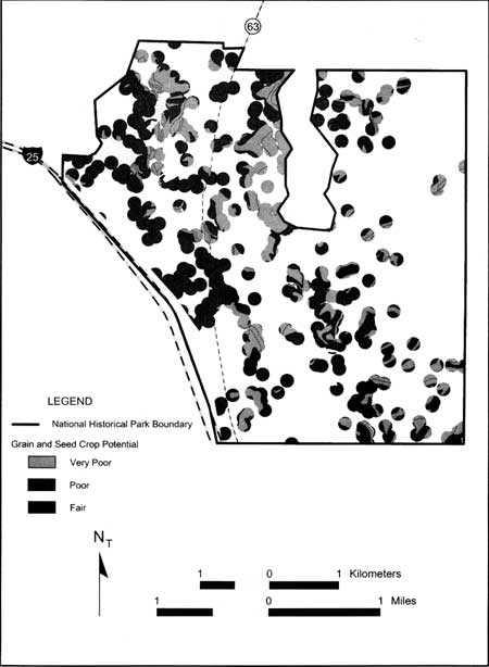
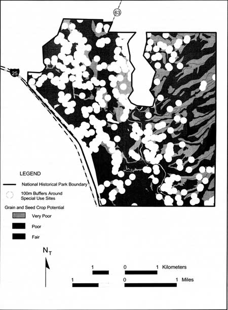
To determine if there are significant associations between the site types and localized plant productivity, a categorical data analysis was performed in which the areas of different plant productivity classes within 100-m of all sites of a particular type were compared to the areas of those productivity classes farther than 100-m from the sites. This was accomplished by generating 100-m buffers around all the sites of each type (illustrated in Figure 6.34 for special-use sites). This buffering process separates the survey area into two classes—those areas within 100-m of sites and those areas more than 100-m from sites (illustrated in Figure 6.35 for special-use sites).
|
| Figure 6.34. Grain and seed potential for areas within 100-m of special-use sites. (click on image for an enlargement in a new window) |
|
| Figure 6.35. Grain and seed potential for areas more than 100 m from special-use sites. (click on image for an enlargement in a new window) |
Statistical Considerations
The analysis presented here utilizes categorical data analysis techniques to determine the degree and character of influence that localized plant productivity had on the selection of prehistoric activity locations. Categorical data analysis is appropriate because of the nature of the data being analyzed. These data represent the areal extent (originally in m2 and converted to 400 m2 blocks [see below]) of different classes of plant productivity within and outside the 100-m buffer defined around each of the different site types. These data are presented most effectively as frequencies within a hierarchical cross-tabulation in which each variable is a column, and each unique combination of values is represented by a row. Each row also presents summary information for each combination of values—the combined areal extent of soil polygons with a unique combination of productivity values, for example. Cross tabulations of this type are illustrated in Tables 6.5, 6.6, and 6.7, in which the productive potential for the food classes are subdivided into those areas within and outside the 100-m buffer defined for habitation sites, special-use sites, and seasonal sites, respectively. These tables differ from standard two-way cross tabulations in that they represent the intersection of more than two variables, necessitating the use of a nested structure for representing the frequencies for each unique combination of variable values (excluding combinations that do not occur in the dataset). Each soil polygon in the study area has a value for each of the three plant productivity classes in addition to an areal extent (in m2). The combined areal extent for each combination of values is presented in the fourth and fifth columns of each table. In the analysis that follows, these calculated areas are used as the foundation of the statistical analysis.
| Table 6.5. Area of plant productivity classes within and outside the
100-m buffer defined for habitation sites. | |||||
| Plant Productivity Potential |
Area (m2) | ||||
| Grain | Herbaceous | Grasses | Within 100-m Buffer | Outside 100-m Buffer |
Total |
| Very Poor | Poor | Very Poor | 75,949 | 7,079,172 | 7,155,121 |
| Poor | 9,113 | 483,408 | 492,521 | ||
| Fair | Very Poor | 9,670 | 191,859 | 201,529 | |
| Fair | 9,763 | 236,512 | 246,275 | ||
| Good | Very Poor | 767,111 | 767,111 | ||
| Poor | Poor | Poor | 7,726 | 282,056 | 289,782 |
| Fair | 13,013 | 334,628 | 347,641 | ||
| Fair | Poor | 5,109,412 | 5,109,412 | ||
| Fair | 99,193 | 5,824,582 | 5,923,775 | ||
| Good | Fair | 28,761 | 2,633,369 | 2,662,130 | |
| Fair | Good | Fair | 328,807 | 328,807 | |
| Good | 145,176 | 145,176 | |||
| Total | 253,188 | 23,416,192 | 23,669,280 | ||
| Table 6.6. Area of plant productivity classes within and outside the
100-m buffers defined for special-use sites. | |||||
| Plant Productivity Potential |
Area (m2) | ||||
| Grain | Herbaceous | Grasses | Within 100-m Buffer | Outside 100-m Buffer |
Total |
| Very Poor | Poor | Very Poor | 2,366,418 | 4,788,703 | 7,155,121 |
| Poor | 171,270 | 321,251 | 492,521 | ||
| Fair | Very Poor | 54,225 | 147,304 | 201,529 | |
| Fair | 93,197 | 153,077 | 246,274 | ||
| Good | Very Poor | 121,229 | 645,882 | 767,111 | |
| Poor | Poor | Poor | 81,401 | 208,380 | 289,781 |
| Fair | 60,758 | 286,883 | 347,641 | ||
| Fair | Poor | 1,483,000 | 3,626,411 | 5,109,411 | |
| Fair | 2,266,409 | 3,657,366 | 5,923,775 | ||
| Good | Fair | 1,001,271 | 1,660,859 | 2,662,130 | |
| Fair | Good | Fair | 23,896 | 304,910 | 328,806 |
| Good | 31,115 | 114,061 | 145,176 | ||
| Total | 7,754,289 | 15,915,187 | 23,669,276 | ||
| Table 6.7. Area of plant productivity seasonal sites. | |||||
| Plant Productivity Potential |
Area (m2) | ||||
| Grain | Herbaceous | Grasses | Within 100-m Buffer | Outside 100-m Buffer |
Total |
| Very Poor | Poor | Very Poor | 1,233,512 | 5,921,610 | 7,155,122 |
| Poor | 185,787 | 306,734 | 492,521 | ||
| Fair | Very Poor | 107,747 | 93,781 | 201,528 | |
| Fair | 120,491 | 125,784 | 246,275 | ||
| Good | Very Poor | 6,634 | 760,477 | 767,111 | |
| Poor | Poor | Poor | 88,042 | 201,740 | 289,782 |
| Fair | 72,207 | 275,434 | 347,641 | ||
| Fair | Poor | 443,222 | 4,666,190 | 5,109,412 | |
| Fair | 1,837,461 | 4,086,314 | 5,923,775 | ||
| Good | Fair | 381,267 | 2,280,863 | 2,662,130 | |
| Fair | Good | Fair | 328,807 | 328,807 | |
| Good | 17,016 | 128,160 | 145,176 | ||
| Total | 4,493,386 | 19,175,894 | 23,669,280 | ||
Two classes of statistical analysis are commonly used to analyze multiway tables—multiple analyses/comparisons and inultivariate methods. Multiple analyses/comparisons entail the analysis of multiple pairings of variables to identify significant associations between pairs of variables in the analysis. There is some question, however, about the utility of the results of the multiple paired analyses for two reasons. First, there is the possibility that some of the identified associations are the result of associations between variables not specifically modeled in the analyses. Without simultaneous consideration of the possible interactions of all of the variables in the analysis, there is always the possibility that identified interactions are the result of unexamined relationships between variables.
The second reason for questioning multiple comparisons is that when the number of analyses increases, the likelihood increases of identifying a significant association when none exists. This is a simple result of the definition of a significance level for a given analysis. For example, if twenty comparisons are performed at a .05 significance level, it is likely that at least one of those comparisons will be significant when it is not, purely as a result of sampling error. While there are methods to control for this effect, it is best to minimize the number of comparisons (Manly 1994:43-44).
Multivariate statistical methods simultaneously consider more than two variables, allowing a single model to quantify the influence of individual variables while also quantifying the interaction among all of the variables. Because of this characteristic, inultivariate statistical methods allow the development of more realistic models. For example, it is more realistic to develop a single model in which localized productivity of multiple resources is considered, as opposed to multiple models in which single resources are considered. Finally, inultivariate methods allow the explicit development of alternative models of the relationships between variables in the context of the known associations among other variables. For these reasons, a inultivariate categorical log-linear analysis is used here (Sokal and Rohlf 1995:743-760).
Log-linear analysis is commonly used with multivariate categorical data. Its primary advantage is that it yields a model for the expected frequencies within a multiway contingency table that can separate the effects of the column and row variables (i.e., the variation in frequencies that is solely dependent upon the values of each individual variable) from the effects of their interaction (i.e., the dependence of expected frequencies on some degree of interaction between the variables). Such partitioning allows for testing the null hypothesis that the variables in the analysis are independent of each other. Furthermore, a custom model for some set of "base" effects can be developed, against which the observed frequencies can be compared (Reynolds 1977:57-79). The comparison of expected frequencies to observed is the basis for the chi-square test. The main difference is that in log-linear analysis the expected frequencies can be calculated using any number of different models, depending on the theoretical underpinnings of the particular analysis, as opposed to the single model used in chi-square analysis. Furthermore, log-linear analyses allow for the development of models in which the simultaneous interaction of multiple variables can be considered and quantified (Fienberg 1977:47-76).
Since this analysis is concerned with the relationship between activity location and localized productivity, it is necessary to focus on the specific interactions between site location and localized plant productivity while controlling for the interactions between the different plant productivity values, independent of activity location. Here, this goal is accomplished by including plant productivity interaction (e.g., the interaction between grain/seed potential and grass potential, or the interaction between coniferous and shrub potential) in the "base" (null hypothesis) model in which site location is assumed to be independent of localized plant productivity.
The Models Considered in the Current Analysis
The null-hypothesis (Ho) for each of these analyses is that there are no significant associations between soil plant productivity and site location. More specifically, Ho is that the variation in the observed frequencies (e.g., the observed areas summarized in columns four and five in Tables 6.5-6.7) can be explained by random variation within each variable and the interaction between the vegetation variables.1 If this cannot account for a significant proportion of the variation in the observed frequencies in the contingency table, Ho may be rejected. If Ho is rejected, further analysis of the data can lead to the development of alternative models that include the interaction between the plant productivity variables and site location.
The likelihood-ratio chi-square statistic (G2) is used to measure the "goodness of fit" between the expected frequencies generated by the null-hypothesis model and the observed frequencies (SPSS Inc. 1999:177).2 To reject Ho, the p value of G2 should be less than the significance level defined for this analysis: =.05. If Ho is rejected, one can conclude that there are additional factors contributing to variability in the frequencies.
To identify meaningful associations between localized plant productivity and site location, an analysis of the adjusted residuals ("residuals") for the Ho model (against the observed frequencies) was performed for each of the six analyses reported below (residuals are the difference between expected and observed frequencies). In each case the residuals were examined for directional trends indicating significant associations between plant productivity and site location. Residuals that exceed a 95 percent confidence interval around the mean (i.e., ± 1.96 standard deviation units) are significant, while their directions indicate the direction of the deviation (i.e., negative values = lower than expected frequencies, positive values = greater than expected frequencies). The deviations from expected frequencies provide the foundation for the interpretations that follow.3
The Analysis Procedure
The first step in the analysis was to generate 100-m buffers around each site within each site type using the buffer.ave script in ArcView 3.0a and a site location GIS coverage generated from the UTM coordinates for the sites. The buffers were then used to extract soil data from a GIS coverage of the soil polygons for the majority of the archeological survey area (e.g., Figure 6.33). This extraction yielded two complementary GIS coverages, one containing soil data for the polygons (or portions of polygons) within the 100-m buffer zone, and one with soil data for the polygons outside the 100-m buffer zones (e.g., Figures 6.36-6.38).
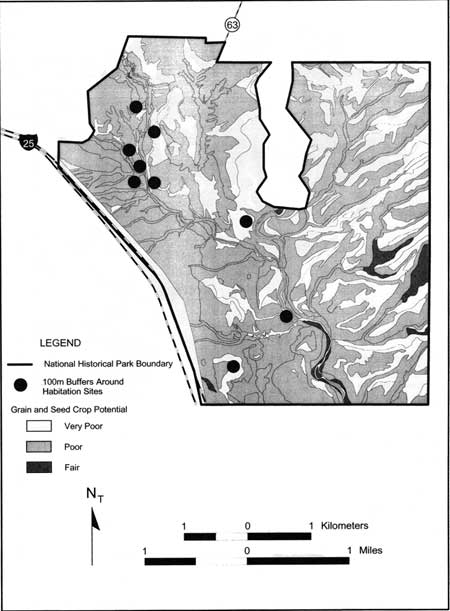
|
| Figure 6.36. 100-m buffers around habitation sites, with grain and seed potential productivity. (click on image for an enlargement in a new window) |
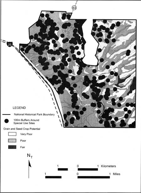
|
| Figure 6.37. 100-m buffers around special-use sites, with grain and seed potential productivity. (click on image for an enlargement in a new window) |
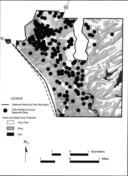
|
| Figure 6.38. 100-m buffers around seasonal sites, with grain and seed potential productivity. (click on image for an enlargement in a new window) |
To provide a spatial scale in line with the sampling strategy used in the survey, the raw areas (in m2) of each polygon in the analysis were converted into an equivalent number of 400 m2 sampling blocks. These blocks correspond with the 10 to 30-m interval used in the archeological survey (averaged to 20-m intervals) and have the effect of subdividing the survey area into 20-x-20-m blocks superimposed on each of the soil polygons. This procedure allows for an explicit definition of the spatial domain for the analysis, mitigating the effects of sample size on the length of the confidence intervals for the parameter estimates in the various models employed.
To determine the best model for explaining the variation in cell frequencies (weighted by the number of 400 m2 blocks calculated for each polygon), Model Selection Log-linear Analyses (using the SPSS hilog procedure) were performed using backward selection. These analyses identified the minimum number of variables (and their interactions) necessary to sufficiently explain the cross-tabulation frequency variation. After verifying that each "best" model required at least one interaction variable above and beyond those represented by Ho (as defined above) and noting which interaction variables were included in the "best" model, the SPSS genlog procedure was run using the Ho model (based on a multinomial log-linear model). The genlog procedure yielded expected frequencies and residuals (among other variables) for each cell in the cross tabulation.
Residuals represent the difference between the observed and expected frequencies for each cell in the cross tabulation and are adjusted to be standardized to a mean of 0 and standard deviation of 1. With a significance level of =.05, residuals greater than 1.96 or less than -1.96 are significant, warranting further examination.
Analysis Results
The results reported herein consist of six separate analyses, two for each of the three site types (habitation, special use, and seasonal)—one for food resources and one for fuel resources. Each discussion outlines the significant interactions between plant productivity and site locations. The residuals are analyzed, focusing on the direction and magnitude of deviations from the expected frequencies derived from the Ho of no significant association between plant productivity and site location. The first presentation of the results (that for food resources at habitation sites) includes an assessment of the interactions resulting from the Model Selection Log-linear analysis. These steps were followed for all analyses. The results are presented in tables but are outlined in the text only once as an example.
Habitation Sites — Food Resources
The results of the Model Selection Log-linear analysis (hilog) suggest that significant interactions exist (above and beyond those between the plant productivity variables) between the following groups of variables:
Areas Within/Outside 100-m buffer * Grasses * Herbaceous
Areas Within/Outside 100-m buffer * Grain and Seed
Areas Within/Outside 100-m buffer * Grasses
Areas Within/Outside 100-m buffer * Herbaceous
The results suggest that there are significant differences between the frequencies predicted by the model associated with Ho (Ho:G2 = 0) and those observed. Since the hilog procedure indicates that there are significant interactions beyond those specified in Ho, the genlog procedure was run for the Ho model to calculate a p value for Ho and to generate expected frequencies and residuals for Ho. The p value for Ho was <.0001 (G2 = 503.7077, df = 35, p value = 2*10-64), confirming the results of the hilog procedure, and indicating that Ho can be rejected. These results are summarized in Table 6.8.
The residuals (Table 6.9) for the Ho model show the following patterns:
The observed frequencies within the buffer are higher than expected (given the Ho model) for the relatively low and middle values for grain and seed productivity, grass productivity, and herbaceous productivity.
Correspondingly, the observed frequencies within the buffer are lower than expected for the relatively high values for grain and seed productivity, grass productivity, and herbaceous productivity.
These patterns suggest that habitation sites tend to be in locations with relatively low potential food productivity within their immediate area.
| Table 6.8. Analysis results summary,
habitation sites and food resources. | |||
| G2 | df | p value | result |
| 503.7077 | 35 | 2*10-64 | reject Ho (G2=0) |
Significant Site Location and Plant Productivity Interactions:
| |||
| Table 6.9. Observed frequencies, expected frequencies, and adjusted
residuals for the localized food resource analysis for habitation
sites. | ||||||||||||
| Within/Outside Buffer | Grain | Grasses | Herbaceous | Observed Frequency |
Ho Expected Frequency |
Ho Adjusted Residuala | ||||||
| Within 100-m Buffer | Very Poor | Very Poor | Poor | 189.87 | 191.34 | -0.13 | ||||||
| Fair | 24.17 | 5.39 | 8.17 | |||||||||
| Poor | Poor | 22.78 | 13.17 | 2.69 | ||||||||
| Fair | Fair | 24.41 | 6.59 | 7.02 | ||||||||
| Poor | Poor | Poor | 19.31 | 7.75 | 4.20 | |||||||
| Fair | Poor | 32.53 | 9.30 | 7.72 | ||||||||
| Fair | 247.98 | 158.42 | 8.26 | |||||||||
| Good | 71.90 | 71.19 | 0.09 | |||||||||
| Outside 100-m Buffer | Very Poor | Very Poor | Poor | 17,697.93 | 17,696.43 | 0.13 | ||||||
| Fair | 479.65 | 498.43 | -8.17 | |||||||||
| Good | 1,917.78 | 1,897.26 | 4.63 | |||||||||
| Poor | Poor | 1,208.52 | 1,218.13 | -2.69 | ||||||||
| Fair | Fair | 591.28 | 609.10 | -7.02 | ||||||||
| Poor | Poor | Poor | 705.14 | 716.70 | -4.20 | |||||||
| Fair | 12,773.53 | 12,636.87 | 13.28 | |||||||||
| Fair | Poor | 836.57 | 859.81 | -7.72 | ||||||||
| Fair | 14,561.45 | 14,651.00 | -8.26 | |||||||||
| Good | 6,583.42 | 6,584.12 | -0.09 | |||||||||
| Fair | Fair | Good | 822.02 | 813.22 | 3.00 | |||||||
| Good | Good | 362.94 | 359.06 | 1.99 | ||||||||
| ||||||||||||
Habitation Sites—Fuel Resources
The null hypothesis (Ho) of no relationship between fuel resource productivity and habitation site locations was rejected (Table 6.10). An examination of the residuals (Table 6.11) for the Ho model shows the following patterns:
The observed frequencies are higher than expected for relatively high levels of coniferous production, while the observed frequencies are lower than expected for moderate and low conifer production potential.
The hilog procedure yielded a "best" model that excluded any interaction between shrubs and the within/outside buffer variable, indicating that no significant association exists between these two variables. Shrub species, therefore, do not contribute significantly to the association between habitation site locations and fuel wood availability.
Overall, these results suggest that there is a significant positive relationship between areas of high potential coniferous production and habitation sites, leading to the conclusion that the availability of fuel wood, or perhaps building materials, influenced habitation site locations.
| Table 6.10. Analysis results summary, habitation sites and fuel resources. | |||
| G2 | df | p value | result |
| 457.1269 | 8 | 1*10-93 | reject Ho (G2=0) |
Significant Site Location and Plant Productivity Interactions:
| |||
Seasonal Sites—Food Resources
The null hypothesis (Ho) of no relationship between food resource productivity and seasonal site locations was rejected (Table 6.12). An examination of the residuals (Table 6.13) for the Ho model shows the following patterns:
Relative to grain and seed production potential, the areas within 100-m of seasonal sites show a mixed pattern of association (some specific cases of higher than expected frequencies, some specific cases of lower than expected frequencies) with relatively low and intermediate values, and consistently lower than expected frequencies with high values of grain and seed productivity.
A similar pattern emerges when grass production is considered. There are mixed patterns of association for relatively low and intermediate values of grass production, while there are consistently lower than expected frequencies for higher values of grass production.
Herbaceous production exhibits a different pattern than that observed for grains and seeds, or grasses. Specifically, the areas within 100-m of seasonal sites generally have higher than expected frequencies for relatively low and intermediate values of herbaceous productivity and lower than expected frequencies for the highest values of herbaceous productivity.
These results suggest that, in general, seasonal sites show the clearest association with locations that have relatively low to moderate potential for herbaceous species, while also showing weaker (in terms of clarity of patterning) associations with low to moderate values for grains and seeds and grasses.
| Table 6.11. Observed frequencies, expected frequencies, and residuals
for the localized fuel resource analysis for habitation sites. | |||||||||||
| Within/Outside Buffer | Coniferous | Shrubs | Observed Frequency | Ho Expected Frequency |
Ho Adjusted Residuala | ||||||
| Within 100-m Buffer | Very Poor | Poor | 111.75 | 103.64 | 0.93 | ||||||
| Good | Good | 280.52 | 128.89 | 16.39 | |||||||
| Outside 100-m Buffer | Very Poor | Poor | 9,419.51 | 9,427.59 | -0.93 | ||||||
| Fair | Fair | 12,773.53 | 12,634.60 | 14.75 | |||||||
| Good | 1,917.78 | 1,896.92 | 4.72 | ||||||||
| Good | Good | 11,573.03 | 11,724.62 | -16.39 | |||||||
| |||||||||||
| Table 6.12. Analysis results summary, seasonal sites and food
resources. | |||
| G2 | df | p value | result |
| 4314.9339 | 35 | 0.0000 | reject Ho (G2=0) |
Significant Site Location and Plant Productivity Interactions:
| |||
Seasonal Sites—Fuel Resources
The null hypothesis (Ho) of no relationship between fuel resource productivity and seasonal site locations was rejected (Table 6.14). An examination of the residuals (Table 6.15) for the Ho model shows the following patterns:
The observed frequencies are higher than expected for relatively high and low levels of coniferous production, while the observed frequencies are lower than expected for moderate conifer production. This pattern is similar to that observed for special-use sites (see below).
There are higher than expected frequencies for relatively high and low productivity values for shrubs within the 100-m buffer areas, while there is a mixed pattern of association for the intermediate values.
| Table 6.13. Observed frequencies, expected frequencies, and residuals for the
localized food resource analysis for seasonal sites. | ||||||||||||
| Within/Outside Buffer | Grain | Grasses | Herbaceous | Observed Frequency |
Ho Expected Frequency |
Ho Adjusted Residuala | ||||||
| Outside 100-m Buffer | Very Poor | Very Poor | Poor | 3,083.78 | 3,395.82 | -7.12 | ||||||
| Fair | 269.37 | 95.65 | 19.82 | |||||||||
| Good | 16.58 | 364.07 | -20.57 | |||||||||
| Poor | Poor | 464.47 | 233.75 | 16.94 | ||||||||
| Fair | Fair | 301.23 | 116.88 | 19.04 | ||||||||
| Poor | Poor | Poor | 220.10 | 137.53 | 7.87 | |||||||
| Fair | 1,108.06 | 2,424.93 | -33.55 | |||||||||
| Fair | Poor | 180.52 | 164.99 | 1.35 | ||||||||
| Fair | 4,593.65 | 2,811.43 | 43.13 | |||||||||
| Good | 953.17 | 1,263.45 | -10.29 | |||||||||
| Fair | Good | Good | 42.54 | 68.90 | -3.54 | |||||||
| Within 100-m Buffer | Very Poor | Very Poor | Poor | 14,804.02 | 14,491.96 | 7.12 | ||||||
| Fair | 234.45 | 408.18 | -19.82 | |||||||||
| Good | 1,901.19 | 1,553.70 | 20.57 | |||||||||
| Poor | Poor | 766.84 | 997.55 | -16.94 | ||||||||
| Fair | Fair | 314.46 | 498.80 | -19.04 | ||||||||
| Poor | Poor | Poor | 504.35 | 586.92 | -7.87 | |||||||
| Fair | 11,665.47 | 10,348.59 | 33.55 | |||||||||
| Fair | Poor | 688.58 | 704.11 | -1.35 | ||||||||
| Fair | 10,215.78 | 11,997.99 | -43.13 | |||||||||
| Good | 5,702.16 | 5,391.87 | 10.29 | |||||||||
| Fair | Fair | 822.02 | 665.96 | 13.98 | ||||||||
| Good | 320.40 | 294.04 | 3.54 | |||||||||
| ||||||||||||
| Table 6.14. Analysis results summary, seasonal sites and fuel
resources. | |||
| G2 | df | p value | result |
| 3640.0023 | 8 | 0.0000 | reject Ho (G2=0) |
Significant Site Location and Plant Productivity Interactions:
| |||
The patterns indicated by the residuals suggest that there may be some overlap between the food resource and fuel wood analyses, specifically in reference to the collection of fuel resources and the selection of locations that are low in conifer density. Low conifer density would facilitate clearing agricultural fields. The higher than expected frequencies for the extreme values for coniferous production within the 100-m buffers and lower than expected frequencies for intermediate values may represent two different patterns of association within this class of sites. First, one set of sites is associated with high productivity conifer areas, perhaps for collecting fuel or construction materials. Second, another set of sites is associated with low coniferous productivity, perhaps indicating a preference for areas requiring less labor to clear and prepare agricultural fields.
Special-Use Sites—Food Resources
The null hypothesis (Ho) of no relationship between food resource productivity and special-use site locations was rejected (Table 6.16). An examination of the residuals (Table 6.17) for the Ho model suggests the following patterns:
The observed frequencies within the buffer are higher than expected (given the Ho model) for some of the relatively intermediate values of grain and seed productivity, otherwise, they are lower than expected for relatively low and high values for grain and seed productivity.
The observed frequencies within the buffer are higher than expected for the relatively middle and high-middle values for productivity of grasses. There are corresponding lower than expected frequencies for the highest and lowest values for grasses productivity.
There are higher than expected frequencies for relatively intermediate values of herbaceous productivity within the buffers, while there are lower than expected frequencies at the lower and upper extremes in potential productivity.
Overall, special-use sites are most frequently associated with intermediate values for all three categories of food resources than would be expected from a random distribution of sites relative to these resources.
| Table 6.15. Observed frequencies, expected frequencies, and residuals
for the localized fuel resource analysis for seasonal sites. | |||||||||||
| Within/Outside Buffer | Coniferous | Shrubs | Observed Frequency | Ho Expected Frequency |
Ho Adjusted Residuala | ||||||
| Within 100-m Buffer | Very Poor | Poor | 2,343.94 | 2,041.40 | 8.81 | ||||||
| Fair | Fair | 1,108.06 | 2,735.83 | -43.68 | |||||||
| Good | 16.58 | 410.75 | -22.55 | ||||||||
| Good | Good | 4,258.19 | 2,538.79 | 46.98 | |||||||
| Outside 100-m Buffer | Very Poor | Poor | 7,187.33 | 7,489.85 | -8.81 | ||||||
| Fair | Fair | 11,665.47 | 10,037.69 | 43.68 | |||||||
| Good | 1,901.19 | 1,507.03 | 22.55 | ||||||||
| Good | Good | 7,595.35 | 9,314.75 | -46.98 | |||||||
| |||||||||||
| Table 6.16. Analysis results summary, special-use sites and food
resources. | |||
| G2 | df | p value | result |
| 1096.1850 | 35 | 2*10-207 | reject Ho (G2=0) |
Significant Site Location and Plant Productivity Interactions:
| |||
| Table 6.17. Observed frequencies, expected frequencies, and residuals for the localized food resource
analysis for special-use sites. | ||||||||||||
| Within/Outside Buffer | Grain | Grasses | Herbaceous | Observed Frequency |
Ho Expected Frequency |
Ho Adjusted Residuala | ||||||
| Within 100-m Buffer | Very Poor | Very Poor | Poor | 5,916.05 | 5,860.14 | 1.07 | ||||||
| Fair | 135.56 | 165.05 | -2.81 | |||||||||
| Good | 303.07 | 628.27 | -16.08 | |||||||||
| Poor | Poor | 428.18 | 403.38 | 1.52 | ||||||||
| Fair | Fair | 232.99 | 201.70 | 2.70 | ||||||||
| Poor | Poor | Poor | 203.50 | 237.33 | -2.69 | |||||||
| Fair | 3,707.50 | 4,184.68 | -10.16 | |||||||||
| Fair | Poor | 151.90 | 284.72 | -9.67 | ||||||||
| Fair | 5,666.02 | 4,851.65 | 16.47 | |||||||||
| Good | 2,503.18 | 2,180.32 | 8.95 | |||||||||
| Fair | Fair | Good | 59.74 | 269.30 | -15.68 | |||||||
| Good | Good | 77.79 | 118.90 | -4.61 | ||||||||
| Outside 100-m Buffer | Very Poor | Very Poor | Poor | 11,971.76 | 12,027.65 | -1.07 | ||||||
| Fair | 368.26 | 338.77 | 2.81 | |||||||||
| Good | 1,614.70 | 1,289.50 | 16.09 | |||||||||
| Poor | Poor | 803.13 | 827.92 | -1.52 | ||||||||
| Fair | Fair | 382.69 | 413.98 | -2.70 | ||||||||
| Poor | Poor | Poor | 520.95 | 487.12 | 2.69 | |||||||
| Fair | 9,066.03 | 8,588.84 | 10.16 | |||||||||
| Fair | Poor | 717.21 | 584.38 | 9.67 | ||||||||
| Fair | 9,143.42 | 9,957.77 | -16.47 | |||||||||
| Good | 4,152.15 | 4,475.00 | -8.95 | |||||||||
| Fair | Good | Good | 762.28 | 552.72 | 15.68 | |||||||
| Good | Good | 285.15 | 244.04 | 4.61 | ||||||||
| ||||||||||||
Special-Use Sites—Fuel Resources
The null hypothesis (Ho) of no relationship between fuel resource productivity and special use site locations was rejected (Table 6.18). An examination of the residuals (Table 6.19) for the Ho model suggests the following patterns:
The observed frequencies are higher than expected for relatively high and low levels of coniferous production, while the observed frequencies are lower than expected for moderate conifer production.
Frequencies are higher than expected for relatively high and low productivity values for shrubs within the 100-m buffer areas, while there is a mixed pattern of association for the intermediate values.
The patterns indicated by the residuals suggest that for special-use sites there also may be some overlap between the food resource and fuel wood analyses, specifically in reference to the collection of coniferous food resources and food resources that may not coexist well with coniferous species. The higher than expected frequencies for the extreme values of coniferous production within the 100-m buffers and lower than expected frequencies for intermediate values may represent two different patterns of association within this class of sites. First, one set of sites is associated with relatively high productivity conifer areas, perhaps for collecting arboreal food resources or fuel wood. Second, another set of sites is associated with low conifer productivity, perhaps for collecting food resources that do not coexist with coniferous species. Without a more detailed analysis that works with mapped productivity potentials at the individual plant species level and more specific information on activities at sites than can be derived from the site typology, it is difficult to assess these potential explanations for the observed patterns.
| Table 6.18. Analysis results summary, special-use
sites and fuel resources. | |||
| G2 | df | p value | result |
| 471.0905 | 8 | 2*101*10-96 | reject Ho (G2=0) |
Significant Site Location and Plant Productivity Interactions:
| |||
| Table 6.19. Observed frequencies, expected frequencies, and residuals for the
localized fuel resource analysis for special-use sites. | |||||||||||
| Within/Outside Buffer | Coniferous | Shrubs | Observed Frequency | Ho Expected Frequency |
Ho Adjusted Residuala | ||||||
| Within 100-m Buffer | Very Poor | Poor | 3,264.29 | 3,082.47 | 4.64 | ||||||
| Fair | Fair | 3,707.50 | 4,131.04 | -9.97 | |||||||
| Good | 303.07 | 620.22 | -15.91 | ||||||||
| Good | Good | 4,392.41 | 3,833.51 | 13.39 | |||||||
| Outside 100-m Buffer | Very Poor | Poor | 6,266.97 | 6,448.77 | -4.64 | ||||||
| Fair | Fair | 9,066.03 | 8,642.45 | 9.97 | |||||||
| Good | 1,614.70 | 1,297.55 | 15.91 | ||||||||
| Good | Good | 7,461.13 | 8,020.00 | -13.39 | |||||||
| |||||||||||
Conclusions
This analysis has examined the relationship between localized food and fuel wood resource productivity and site locations. The results indicate that there are significant relationships between localized plant productivity and site locations for all three site types. While the direction and magnitude of the relationships vary from analysis to analysis, in all but one case, all of the variables included in the analysis made a significant contribution to the variance in frequencies observed in cross tabulations generated for each analysis. The exception was the one between habitation locations and fuel wood resources, in which the productivity of only one of the two plant types was significant. Furthermore, each of the analyses indicated that there are significant associations between the different classes of plant productivity, independent of site location, which reaffirms the choice of a multivariate approach.
The patterns of association for habitation site locations can be summarized as follows:
Habitation site locations are associated with areas of relatively low food resource potential.
Habitation site locations are associated with relatively high coniferous resource potential, indicating a preference for areas with high fuel wood, or perhaps construction material, potentials.
The results of the analysis of seasonal site locations can be summarized as follows:
Seasonal site locations are most clearly associated with low herbaceous potentials, while showing mixed results for grain and seeds and grasses.
Seasonal sites are positively associated with high and low potentials for coniferous and shrub species and negatively associated with intermediate potentials for these species.
The results of the analysis of special-use site locations can be summarized as follows:
Special-use sites are more frequently found in locations with intermediate plant productivity for all three classes of food resources, while the frequencies for high and low potentials are lower than expected.
There are higher than expected associations with high and low values for both shrubs and conifers, and lower than expected frequencies for intermediate shrub and conifer productivity.
The overall results of this analysis suggest that the relationships between site locations and plant productivity are significant and complex. Habitation sites clearly are associated with areas of low food plant productivity and high wood productivity. This indicates that habitation sites are specifically situated to minimize impact on productive food patches, while also providing convenient access to fuel and construction materials.
The relationships between seasonal and special-use sites and localized plant productivity indicate that simple models which assume these activity locations map onto areas of high productivity may be inadequate. The association of seasonal sites with low herbaceous productivity and mixed association with the other food resource categories suggest that factors other than localized food production play a role in the placement of these sites. Similarly, the association of special-use sites with intermediate productivity values for the three food resource classes also indicates that factors other than food resource productivity are making a significant contribution to the decision-making process associated with the placement of these sites.
In summary, this analysis has provided a more detailed assessment of the contribution of plant resources to variation in site location in the survey area than could be derived from current vegetation patterns. While not providing a complete explanation for the locations of sites on the landscape, these results, when combined with the results of complementary analyses, provide a greater understanding of the variables involved in prehistoric land-use decisions. The significant results obtained in this analysis suggest that small-scale spatial analyses have the potential to complement larger-scale analyses, including catchment analyses, when both can be utilized.
Summary and Conclusions
In this chapter we have tried to examine site locations and community development from several different perspectives. Site locations according to elevation and landform indicate a persistent diversity that is contrary to what we expected based on the number of sites in each period and the PDSI dryness index. It appears that diversity is always desirable, probably because there are elements of the social and physical environment that are always unpredictable, and diversity helps smooth the unpredictability. Habitations and seasonal sites often are above 6,600 ft (2,012 m) in elevation, which Snow (1991) considers the upper limit for producing a mature corn crop in New Mexico.
In addition to environmental variables, social conditions also affect site locations. The nearest neighbor analysis was designed to identify social, and to some extent, economic influences on site locations. Nearest-neighbor distances (NND) within and between site types in each period were examined. In two-thirds of the analyses, sites were clustered. Seasonal and special-use sites, both within and between types, were consistently clustered, probably reflecting occurrence of resources and similar environmental conditions conducive to domestic and wild resources. It was clear that resources closest to habitations were used first, and in response to local depletion, nonhabitation sites were moved farther from habitations through time.
When the productive potential of soils in specific site environments was examined it became clear that the different site types were found in areas with distinct characteristics. Habitation site locations are associated with areas of low food resource potential but high coniferous production. It appears that habitations were situated to minimize impact on potentially productive food resources, while being located to exploit wood resources for fuel or construction. Seasonal and special-use sites appear to fall into three classes. Some seasonal and special-use site locations appear to select for food resource potential, while others are significantly associated with high wood resource productivity. Other locations are significantly associated with low conifer and shrub productivity, probably representing areas that are easier to clear for agricultural fields. More specific information on activities at different kinds of sites might elicit clearer relationships with different soil productivity potentials.
Approaching settlement from three different perspectives has allowed us to see that topography (elevation and landform), the proximity of other sites and the character of specific locations are all important aspects of the settlement system in the Upper Pecos Valley. Future research into settlement at Pecos might fruitfully consider further the important role of water in site location, and noneconomic aspects of site placement, as well as the numerous isolated finds recorded by the survey that could not be considered here. Adding these details will more fully flesh out our understanding of the ways the Pecos people created a dynamic cultural landscape that allowed them to survive in an unpredictable world.
Notes
1. Models Used in the Analysis
In mathematical terms, the models used in this analysis can be summarized as follows: The base models represent the model used to calculate the expected frequencies for each cell in the contingency table based upon Ho, while the saturated model (Modelsat) represents a model in which all possible interaction terms are included (which also yields frequencies equal to those observed). If no significant difference is found between the frequencies calculated from the base model and those from the saturated model, Ho is not rejected, and no significant associations between the localized plant productivity values and site location are found. If, on the other hand, significant differences are found between the expected frequencies generated using the base model and those calculated from the saturated model, significant associations between localized productivity and site location may be supported.
G2 = 2ΣiOiIn(Oi/Ei)G2 = Likelihood - Ratio Chi - Square
0/ = Observed Frequency for Cell i
E, = Expected Frequency for Cell
For the Food-Related Variables
Modelbase:In Ei = θ + &lamda;1i + &lamda;2i + &lamda;3i +
&lamda;4i + &lamda;23i + &lamda;24i + &lamda;234i
Modelsat:In E1 = θ + &lamda;1i + &lamda;2i + &lamda;3i +
&lamda;4i + &lamda;23i + &lamda;24i + &lamda;34i + &lamda;234i +
&lamda;12i + &lamda;13i + &lamda;14i + &lamda;123i + &lamda;124i +
&lamda;134i + &lamda;1234i = InOi
&lamda;1 = within /outside buffer, &lamba;2 = grain&seed, &lamda;3 = grasses, &lamba;4 =
herbaceous, &lamda;12 = interaction between within /outside buffer and grain&seed, etc.
For the Fuel-Related Variables
Modelbase:InEi = θ C
Modelsat:In Ei = θ + &lamda;1i + &lamda;2i + &lamda;3i + &lamda;23i +
&lamda;12i + &lamda;13i + &lamda;123i + =In Oi
&lamda;1 = within /outside buffer, &lamba;2 = coniferous, &lamda;3 = shrubs,
&lamda;12 = interaction between within /outside buffer and coniferous, etc.
Modelbase:In Ei = Model used in the calculation of the Ei values for Ho
Modelsat = Saturated model that represents all possible interactions between variables
Ei = Expected Frequency for Cell i
Oi = Observed Frequency for Cell i
θ = constant Term
&lamda;ni = Parameter Representing a Single Variable (e.g. &lamda;1) or the interaction
between variables (e.g. &lamda;12), for Cell i
&lamda;addi = Parameter Representing Term(s) Added to Model to be Tested for Significance for Cell i
2. Calculation of the Likelihood-Ratio Chi-square Statistic
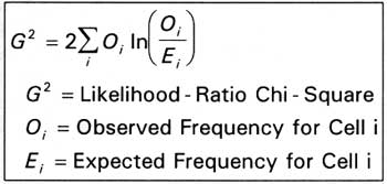
3. This form of descriptive analysis of the residuals is only an approximation of a more detailed analysis that is beyond the scope of this report. This more detailed analysis would calculate log-odds ratios for the different levels between pairs of variables while controlling for interaction terms (Le 1998:95-101). These calculations would yield a more detailed picture of the association between variables of interest but require the calculation of numerous equations.
| <<< Previous | <<< Contents>>> | Next >>> |
peco/cris/chap6.htm
Last Updated: 13-Feb-2006