Geological Survey Professional Paper 1365 Ice Volumes on Cascade Volcanoes: Mount Rainier, Mount Hood, and Mount Shasta

Portable monopulse-radar equipment that could be deployed rapidly from a backpack and antennas applicable to a wide range of ice thickness were needed to complete the work. In the radar operation, separate transmitting and receiving antennas were placed on the ice a known distance apart. An oscilloscope recorded arrival of the transmitted air wave and the wave reflected from the bedrock (fig. 2). Oscilloscope screen output was photographed on self-developing film. The theory and principles of operation of the monopulse radar are described in more detail in the appendix.

FIGURE 2.—Ice radar unit in operation on Diller Glacier on the Middle Sister, Ore. The transmitter and antennas are on the snow. Receiving unit and oscilloscope are operated from top of backpack in photo. (U.S. Geological Survey photograph by Carolyn Driedger in September 1981.)

As all depth measurements were point measurements, it was necessary to obtain accurate map positions, and, as large ice masses have few features identifiable with certainty on a map, surveying was required on Mount Rainier and Mount Hood. Standard survey procedures were followed for field surveying; a theodolite and an electronic distance-measuring device were used. Because glaciers on the Three Sisters and Mount Shasta are generally smaller than those on Mounts Hood and Rainier, locations could be determined adequately with a pocket transit and aerial photos.

Measurement points were selected to give representative coverage of the major ice bodies on each mountain, as well as on some smaller glaciers and patches of perennial snow (firn), referred to in this paper as snow patches.

The number of measurement points on each glacier ranged from l to 31. The ultimate number and locations were determined by weather, avalanche and ice-fall conditions, suitable helicopter landing areas, and the ability to obtain unambiguous bottom-measurement returns. Final data-point locations are shown on plates 1-6.

PRIMARY DATA REDUCTION

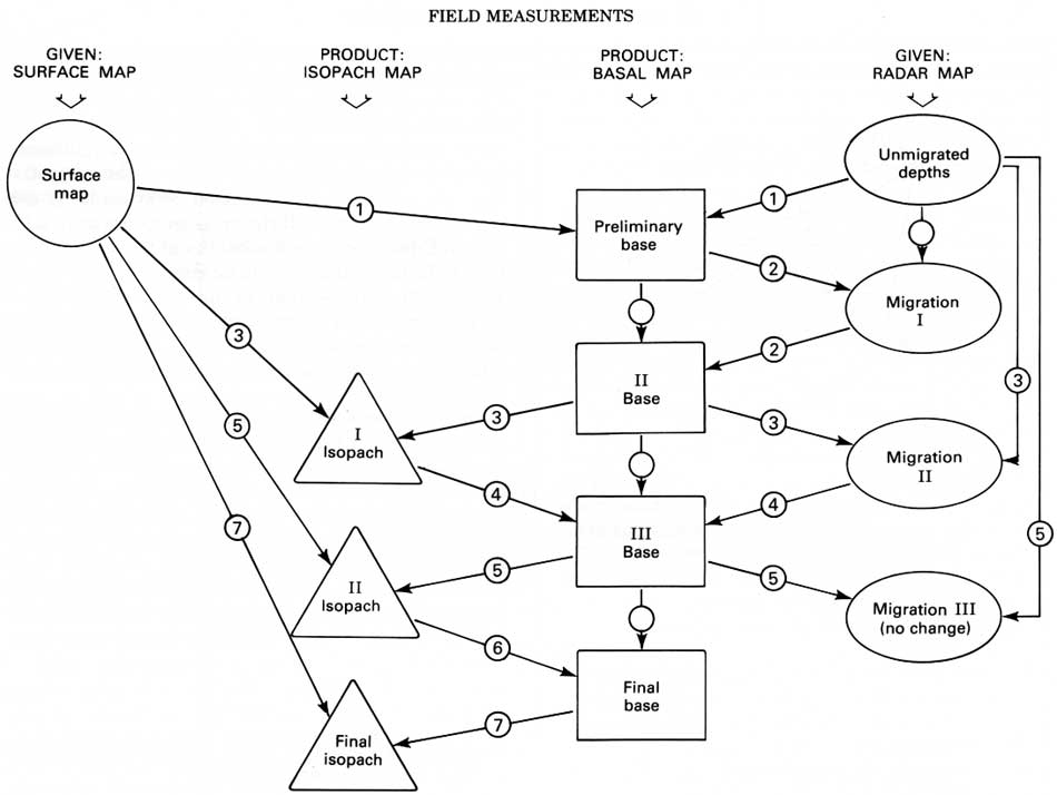
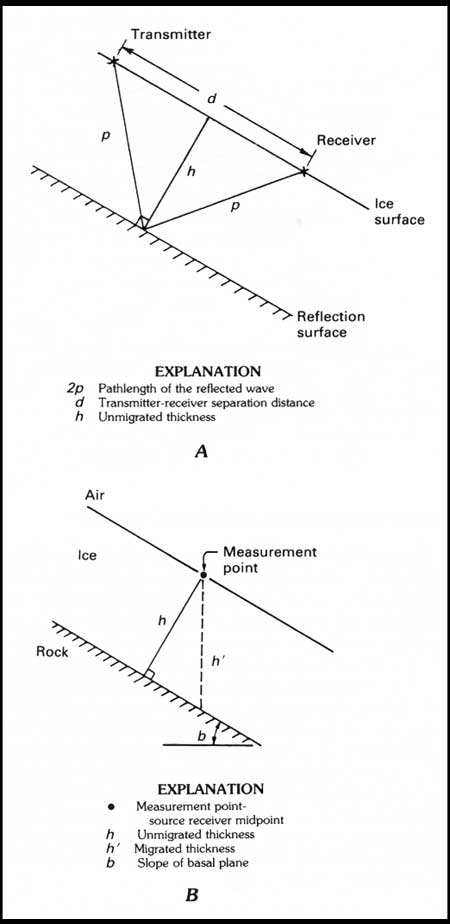
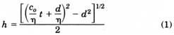
The iteration of processes required for developing bedrock and isopach maps is detailed here and is summarized in figure 3. The first step following fieldwork involves finding the ice thickness at each measurement point. Figure 4 shows the geometry of a measurement point and indicates the path of the radar wave between bedrock and the surface. The procedure uses equation 1, where it is assumed that the glacier and bedrock surfaces are planar and the glacier consists only of ice.

FIGURE 3.—Interactive processes used to produce basal and isopach maps, as in plates 1 through 6 (Kennard, 1983). (click on image for an enlargement in a new window)

FIGURE 4.—A, The location of the transmitter and receiver relative to the bedrock reflection surface. B, Closeup of A that indicates the slope correction necessary for measuring vertical ice thickness rather than distance from the transmitter to the nearest reflection surface (Kennard, 1983).

Required for the calculation are the separation distance between the pulse source and the receiver (d), the time interval between the arrival at the oscilloscope of the air wave and the reflected wave (t), the speed of light in a vacuum (c₀), and the refractive index of ice (η). An apparent thickness (h) was calculated at each point by

Computations showed that correcting for the differences in the refractive index on ice, firn, and snow had an effect of less than two and a half percent on glacier-thickness determinations because the layers of snow and firn are thin. In the data reduction, the presence of snow and firn were disregarded and the total thickness at each measurement point was assumed to be ice. Any debris-laden layer at the base of the ice was assumed to be a reflecting surface and was considered glacier bed.

Thickness measurements were considered accurate to ±3.0 percent for a typical data point, including photograph reading errors and errors owing to neglecting the presence of snow and firn. These apparent point thicknesses, together with geological interpretation, were used to develop subglacial contour maps, referred to hereafter as basal maps.

USE OF MEASURING POINT MIGRATION TO CORRECT FOR BEDROCK SLOPE

Initially, the basal altitude below each measured point was assumed to be the surface altitude less the apparent thickness (fig. 4A). However, because radar reflects off the nearest rock surface, a migration correction is required to find the true thickness vertically beneath each point.

The ice-depth equation (eq. 1) defines an ellipsoid, the radar source and receiver being at the respective foci. Theoretically, the reflection point could lie anywhere on this surface. If the measurements were taken within a distance of each other equal to an ice depth, a true reflection surface could be constructed by the envelope of the intersections of the various ellipsoids. In all but one instance, measurements were too far apart to allow construction of an envelope, and a geometrical migration scheme was required to determine the basal geometry.

For example, with a measurement made on steep ice in the middle of a glacier, the reflection point would most likely come from rock at an angle to the point and not directly below it (fig. 4B). Similarly, a sounding taken on a flat section of glacier near the valley wall would most likely be reflected from the side rather than from directly below. Because a map projection of the glacier was used, knowledge of the vertical distance between the measuring point and the bedrock (h') was required. This was calculated by

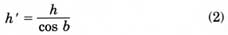
where b was measured along the bedrock slope and through the measurement point.

For purposes of migration only, it is assumed in the above equation that the transmitted radio wave is spherical, hence negligible error for typical readings is introduced. Using the basal map developed with apparent thicknesses, we computed angle b by measuring the distance between contours along a curve perpendicular to the contours and passing through the measurement point.

The apparent thickness was migrated by using this estimate of basal slope in the immediate measurement area to yield an estimated base elevation directly below each measurement point. This was used to revise the basal contour map; a new basal slope was measured and the process repeated. This migration scheme was iterated, usually three or four times, with changes up to several millimeters at the map scale, until the base elevation value ceased changing. When drawing contours around individual measurement points, the estimated thickness was not expected to apply directly to the base area for more than approximately a distance equal to the ice thickness, though its influence on the contour pattern may have extended farther. If a contour were moved during migration, it was generally necessary to adjust the neighboring contours. Ice-surface features seen on aerial photographs were used as an aid in correctly locating the contours.

USE OF MAPS AND PHOTOGRAPHS TO INFER BASAL TOPOGRAPHY

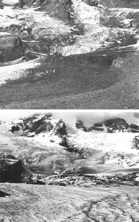
The maps used were the most current U.S. Geological Survey topographic maps available for each area. The Mount Hood, Mount Shasta, and the Three Sisters maps were enlarged to a scale of 1:10,000 and then reduced to 1:20,000 for this publication, and the Mount Rainier map was used at the original scale of 1:24,000 and reduced to 1:48,000 for this publication. Two-hundred-foot contour intervals were used on Mount Rainier and 100-foot intervals were used on the other mountains for ease in determining area and volume by altitude. Observations from photographs were an important part of map development, as they were useful as indicators of basal relief. Where available, some older photographs showing lower ice levels and exposed basal relief were examined (fig. 5).

FIGURE 5.—Two views across Nisqually Glacier toward Wilson Glacier illustrating the use of aerial photographs in determining the location of bedrock. A, Glacier conditions during 1944 permitted exposure of a bedrock cliff in lower Wilson Glacier seen near the center of the photograph; B, The same area with bedrock submerged during 1980. (U.S. Geological Survey photographs by Fred Veatch on September 30, 1944, and by Carolyn Driedger on July 31, 1980.)

Field observations and autumn 1980 and 1981 aerial photographs were used to update the maps for current glacier boundaries, termini positions, and perennial snow patch locations. Therefore, the resulting maps and values indicate areas and volumes in autumn, at the end of the ablation season.

ICE-SURFACE FEATURES AND THEIR RELATION TO THE BASAL TOPOGRAPHY

It is generally accepted that the surficial topography of a glacier reflects bed topography in diminished complexity, though bed features are reflected more accurately on the surface of thin ice than on thick ice. It is possible through the judicious use of photographs to determine the trend of the basal topography for most glaciers.

Bedrock configurations induce flow regimes recognizable by characteristic crevasse patterns, but care must be taken when using these to infer basal topography. Interpretation of the crevasse patterns is necessary to distinguish between those caused by the shear stress along the valley walls and those caused by local relief along the channel. Local changes in slope or channel width lead to areas of extending and compressing flow. Transverse crevasses tend to define areas of extending flow. In general, extending flow occurs above icefalls, and compressing flow occurs below them. Extending flow commonly occurs in accumulation areas. Crosshatched crevasse patterns may arise from ice flow over a bed bulge. A reduction of valley wall constraints often leads to splaying crevasses as seen near glacier termini. Generally, crevasses are products of stresses due to local topographic irregularities in the glacier bed, though they may move with the ice from the area in which they formed.

Some surficial features bear no relation to bedrock topography. Wind-caused features and avalanche deposit zones can result in anomalous surface curvature. Convergent or divergent ice streams may deform the ice; these ice streams are detectable with their accompanying medial moraine, as seen during low-snow-year photography. Kinematic waves, in response to an accumulation perturbation, may cause minor surface bulging independent of base morphology. Interpretation of photographs taken over several years allows identification of these phenomena.

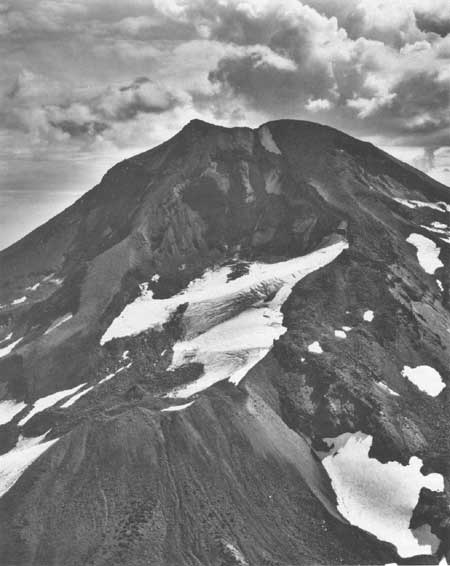
Catastrophic events can have long-term effects on a glacier's surface. The insulation of ice by rockfall results in the appearance of a raised underlying surface, a false indication of bedrock rise. An example of this is at Lost Creek Glacier on the South Sister (fig. 6), where existing maps, showing rockfall debris on the ice as bedrock, incorrectly identify the glacier as two separate ice fields.

FIGURE 6.—Rockfall partly concealing ice (left of center in the photograph), as seen here on Lost Creek Glacier in the Three Sisters, must be identified as such for the proper volume estimation. (U.S. Geological Survey photograph by Austin Post on September 10, 1980.)

The endpoints of each basal contour to be drawn are known at the ice-rock boundary. From basal contours well constrained by radar measurements, it was seen that the exposed valley walls would maintain their configuration for a distance subglacially. This seemed particularly true where the valley wall was very steep in the lower reaches of a well-developed valley glacier. The presence of morainal debris and stream sediment at the glacier terminus was considered in this interpretation.

Despite the use of radar measurements and photographs, data were limited for defining small-scale features in the basal contours. This necessitated smoothing of the contours and the drawing of small-scale features only where strictly warranted by the data.

The primary component of the error is this extrapolation of the local bedrock depths over a large subglacial area. Error made in the interpretation of bedrock topography by use of radar measurements and photographs was calculated at 16 percent. This was calculated by using independent interpretations of bedrock topography made by several glaciologists for South Cascade Glacier, which has a volume well known from previous intensive radar measurements.

ISOPACH MAPS AS INTERPRETIVE TOOLS

Isopach maps (pls. 2 and 5) are derived by the subtraction of altitudes between the surface and migrated basal contours; they indicate areas of equal ice thickness.

Although these values are defined explicitly by the surface-basal maps, the isopach contour connecting them is subject to interpretation. Again, the simplest solution was chosen, with curvature and number of areas bounded minimized. All radar points were checked to assure that they were located in the correct thickness field.

Analyses of isopach maps reveal patterns in the ice thickness that indicate icefalls, rock ribs, and basins or irregularities in the surface-based maps. Therefore, the isopach map became an interactive tool in the process of refining the basal contour maps. For all measured glaciers, a graph that shows thickness as a function of area was prepared (figs. 11, 15, 19, 23).