NATIONAL PARK SERVICE The Impact of Three Exotic Plant Species on a Potomac Island

Design of Observations and Statistics

Survey designs used were census, simple or complete random sampling, paired plots, and model II regression. The experimental designs used in this study were complete randomization (for both two and more groups), paired plots, randomized complete block, Latin square, and model I regression. Except in a very few obvious instances, all data (both discrete and continuous variables) were statistically analyzed. Because statistical analysis of samples is based on homogeneous variance, this was tested either by Bartlett's test or variance ratio test (and in many cases brought into homogeneity by a transformation) before the t test, analysis of variance, analysis of covariance, regression, or chi-square test was applied. The only arc sine transformations made in my study are in degrees not radians. If the variance remained heterogeneous, then a modified t test or other statistical test of comparison was applied. If the variance was on the borderline (usually 0.1 or 0.05). the statistical test of comparison was used both modified and unmodified. The t tests were modified by methods given both by Snedecor and Satterthwaite. For a modified paired t test, the samples were unpaired and considered as equal sample sizes. Modification for a one-way analysis of variance was to set the significance level higher at 0.05 and rely more on the biology, or at 0.005 and rely more on physical conditions. A significant heterogeneity chi-square required reliance on the individual chi-squares. With every analysis of variance or covariance, Duncan's "new multiple range test" was applied when replications were equal, and Kramer's modification was applied when replications were unequal or variances were heterogeneous, or means were correlated. (In the tables, both tests are referred to as Duncan's test.)

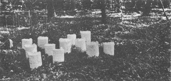
Cheesecloth covered wire frames used for the controlled shade and light experiments with Hedera helix.

Whenever a regression was applied, it was tested for significance and the coefficient of determination (or multiple determination) computed.

Significance levels were set as follows. Because of the variation in biological material in the field, significance levels were set for field experiments as well as surveys at 0.1 (10%). Physical material was expected to vary less; therefore, when only these were involved, significance was set at the 0.01 (1%) level. (One exception was made when published data were analyzed.) For experiments using biological material isolated from its usual surroundings and over which more control could be exercised, the significance level was set at 0.05 (5%). All experiments were replicated at least three times and all surveys were based on at least three replications of the sample unit.

Most of the field experiments and all of the sample survey units were set up at random on the island by use of a random digits table. I consistently used the method described by Phillips (1959:23) for locating starting digits in the table.

The statistical references consulted are listed in the Appendix.

The Physical Setup (Materials)

The Habitats Studied

To answer the questions on exotic impact a well-integrated physical setup was needed since many of the experiments and surveys were performed on a given set of quadrats or points. This will be described and the experimental and survey observational methods related to it.

Each of the three exotic species was studied in two different habitats. Hedera helix was studied on the upland and in the flood plain. Lonicera japonica was studied in an area where the forest understories were intact and in an area where the underbrush had been removed several years ago by the National Park Service; both are on the upland. Iris pseudacorus was studied near the tidal gut and by the tree line (edge of the swamp); both of these areas are in the big marsh.

The Placement of 1 x 1-m Quadrats

After an inventory of all the possible areas, ten blocks of three 1 x 1-m quadrats each were laid out at random on the upland in Hedera helix. The 1-m² plots in each block were laid out 0.5 m apart on the contour by using a tape, surveyor's rod, and level. To assure each block being a valid replication of the others, uniformity of coverage by the exotic was set as close to 100% as possible. This principle applies to all randomized block and paired plot designs. Plots containing much less than complete coverage by the exotic could be used, in theory, but would be hard to replicate. One plot in each block was a control that received no treatment, whereas the other two did. The selection of plots for treatment or controls was by a random digits table; this principle applies to all selection of control and treatment plots. The treatments will be described later. There were, then, 30, 1-m² quadrats, 20 of which received a treatment.

On the flood plain, seven blocks of three 1 x 1-m quadrats each were laid out in Hedera helix plus a placement of one pair of 1 x 1-m plots (one of which was a control plot). This gave 8 control plots and 15 treated ones. For some studies, more were needed and an additional five 1 x 1-m plots were randomly selected. On the flood plain (a flat area), the three plots within each block were laid out on the corners of an equilateral triangle. A minimum of 0.5 m separated the plots at their closest points; this same separation held for the pair. The reason for this mix of designs was the physical impossibility of placing any more complete blocks or pairs in otherwise suitable H. helix; there were too many trees and shrubs in the way. For this area, then, there were 28, 1-m² quadrats.

The placement of plots (1 x 1 m) in Lonicera japonica under a natural understory presented problems similar to those encountered on the flood plain with Hedera helix. Although L. japonica is widespread and abundant, finding areas large enough to place two or three quadrats and have all quadrats be uniformly covered (for valid replication) with the exotic is a problem. For L. japonica under a natural understory, three blocks of three 1 x 1-m plots each were placed. They were laid on the contour as described for H. helix on the upland. An additional five pairs were also laid out on the contour, thus making a total of 19, 1-m² plots, 8 of which were controls and 11 received treatment.

When only two plots of a randomized block layout were used, they were used as paired plots. Whenever possible in the case of mixed designs, analysis was run two ways as a means of verification. For example, part of the data analyzed by randomized block with three replications could be analyzed by paired plot. Eight paired plots (three from the block design and five pairs as originally set up) were used to verify an aspect of the block design.

Ten pairs of 1 x 1-m quadrats were placed at random and on the contour in the Lonicera japonica, which is in the forest area cleared of underbrush. One plot of each pair was randomly selected as a control plot. These also were 0.5 m apart in the pairs.

In the marsh, both near the gut and near the swamp forest edge, some latitude had to be allowed regarding distance between plots within a block or a pair, because in many places, particularly near the gut, Iris pseudacorus grows in clumps often about 1 m² in area. Thus, the plots were often further apart than 0.5 m. In all cases where blocks could be laid out, the plots formed a triangle but not necessarily equilateral. The orientation of each plot was governed by where the Iris was or was not.

In the marsh toward the gut, I laid out all the blocks of three 1 x 1-m plots and paired 1 x 1-m plots that were possible. This resulted in three blocks of three plots each and four pairs of plots. This provided seven control plots and ten plots for treatment. An additional five 1 x 1-m plots were randomly selected, thus giving a total of 22, 1-m² plots for this area.

For the marsh area near the swamp forest line (swamp-marsh transition), I also laid out all the blocks of three plots and all the pairs possible. This resulted in four blocks of three 1 x 1-m plots each and nine pairs of 1 x 1-m plots. This provided 13 control plots and 17 plots for treatment. An additional three 1 x 1-m plots were randomly selected thus giving a total of 33 plots in this area.

Altogether, 152, 1 x 1-m plots were placed in blocks, pairs, or singly in six habitats involving three exotic species and satisfying the randomization needed for statistical analysis. In the forested areas, the corners of the 1 x 1-m plots were marked by nails or spikes about 15 cm long, tied with white cord and driven into the ground. In the marsh these are too short because they tend to sink into the mud too readily. To mark the corners of the marsh plots, spikes 26 cm long and tied with colored surveyor's flagging were used. Around the blocks and paired plots, a simple fence of string with surveyor's colored flagging tied on it was placed to remind park visitors not to walk on the plots. Wooden stakes (2 x 2 inch—or more like 4 x 4 cm) were used as fence posts; sometimes trees were used.

The Placement of Light Stations

An extensive layout of light stations was set up on the island to test the hypothesis that light is a limiting factor in the spread and growth of these three exotic species. To accomplish this, 126 light stations were set up in the following areas for the purposes stated. A light station was established for each block and paired plot. For the blocks that occurred three in a row on the contour, a random digits table was used to determine whether the station should be placed between plots 1 and 2 or between 2 and 3. For blocks with the plots placed on the corners of a triangular area, the station was placed in the middle of the triangle and surrounded by the three plots. Stations were established between paired plots.

Comparisons were made in similar habitats without the exotics. Ten stations were placed at random in the upland forest where exotics were not noticeable and Hedera helix and Lonicera japonica were absent. Another 10 were placed similarly at random on the flood plain. Twenty stations were randomly placed in the marsh where there were no Iris. Ten of these were in the open area and ten in the swamp-marsh transition near and at the tree line. The random placement of these 40 light stations in areas of nonexotic vegetation was accomplished by drawing coordinates at random (from a random digits table) for a grid placed on a map of the island. Because each division of the grid was about 2.3 m, no backsights and only one foresight was taken in the field in locating the points on the ground. This was done to ensure error and hence increase randomization.

All light measurements were compared with open sunlight. For this purpose, 10 randomly placed stations were located in the open field just north of the highway bridge. Coordinates of a grid were placed on the ground in the open area and random coordinates selected by means of a random digits table.

There was some concern that the lights from the highway bridge might influence the light readings. To check this, an additional 20 stations were placed randomly (by using a random digits table) along the four stone railings of the two bridges at the monument to Theodore Roosevelt, which is just north of the center of the island. These bridges are at the northwest and southeast sides of the monument area.

The light meters (Ozalid type) in the forest areas were placed at the height of the vegetation layer beneath the shrub layer at that point; nails, spikes, or metal rods were used to support the meters. Masking tape was used to fasten the meters to the support except where the meter was on the ground; in such cases, three nails driven into the ground around the meter held it in place. In the marsh area and the field, the meters were placed at the height of the tall herb vegetation at that point. Masking tape was used to fasten them to the wooden support stakes. A grease pencil was used to mark the stations on the stone rails of the monument. Because masking tape does not stick well to a wet or damp stone surface, filament tape was placed on the stone when dry and masking tape was used to fasten the meters to the filament tape surface.

To mark the location of the forest light stations and to be able to find them with snow on the ground, if need be, a cord was fastened from the support to some nearby vegetation and a colored ribbon of surveyor's flagging was tied to the cord.

The Ozalid meters are sensitive to wavelengths around 410 mµ (Friend 1961:579).

The Placement of Vegetational Strata Stations

Another means of investigating light was to study the stratification of vegetation in areas where trees and shrubs were present. With the exception of the points on the monument, in the field, and in the marsh away from the swamp-marsh transition zone, the light stations doubled as sampling stations for investigating stratal relationships. In addition, 13 points were established in the swamp in the following manner. A line was laid perpendicular to the tree line closest to the light station in an Iris block or paired plot in the swamp-marsh transition area. This perpendicular line not only passed through the station but also extended to a point away from the marsh and passed obvious Iris until about halfway under the first limb of the first canopy tree. These points were marked with flagged stakes.

The Placement of Elevation Stations

To provide a description of the flood crest, five elevation stations were selected, but not at random. The selection was based on access during the flood as well as a representative sample. In relation to the upland (not flood plain) part of the island, the points were located as follows: northeast, north-northeast, north, west, and southwest. Two other stations were marked, but they disappeared.

The 20 light stations in the marsh not associated with plots plus the centers of the 20 control plots in the marsh were used as elevation stations in relation to investigating water as a limiting factor. In addition, 10 more elevation stations were located on the bank of the tidal gut closest to the non-Iris swamp-marsh transition zone light stations.

The Competition Experiments

Twenty-five wire baskets, 10 cm high, about 22 cm in diameter, and lined with treated paper (for water retention), were placed on a sloping metal roof which is shielded on two sides. These baskets were placed in the form of a square with five baskets on a side and were used in a 5 x 5 Latin square experimental design in an Iris competition study. Holes cut in thin plywood held the baskets about 25 cm apart; C-clamps held the plywood to the roof.

The Germination Observations

Twenty-five cans 17.5 cm high and 10.5 cm in diameter were used for germinating seeds. These were placed in the form of a square and attached to the same roof in the same manner. The center of each can was 30 cm from its neighbor.

The Controlled Shade and Light Experiments

Two sets of experiments with sunlight and degrees of shading were performed: one in a dense stand of Hedera helix, the other in a dense stand of Lonicera japonica. The physical layout for each was as a randomized complete block experiment with a control, and four treatments each of which were replicated 3 times. Each block of five 1 x 1-dm plots was placed on the contour. Two nails about 15 cm long marked the location of the uppermost corners of each plot. Each plot was covered by a wire basket about 22 cm in diameter and 31 cm high. Prongs on the bottom of the baskets about 5 cm long were pressed into the ground to help hold the baskets in place. Except for the controls, the baskets were wrapped in layers of cheesecloth: 12 layers, 24 layers, 48 layers, and 96 layers. When light measurements were taken, the meters, attached to 15-cm nails with masking tape, were placed in the center of each 1-dm² plot. Altogether there were 30 plots each 1 dm².

The Censuses

A census was taken for the three surveys involving Ulmus americana and exotic vines. The total trees involved were 1132.

The Observational Methods

Control Check

All control plots were read for exotic frequency in the spring of 1972 (the observed frequency) and compared with the reading of the same plot in the spring of 1971 (the expected frequency) by a chi-square analysis of 1 x 2 tables. The reading dates were as follows: upland Hedera, 31 March; natural understory Lonicera, 1 April; flood plain Hedera, 1-5 April; open marsh Iris, 2-4 April; swamp-marsh transition Iris, 2-5 April; cleared understory Lonicera, 12 and 13 April. With the exception of the open marsh Iris, the analysis was on the pooled data for all the control plots. The exception, due to heterogeneity (significant beyond 0.001), required analysis of the individual chi-squares for each of the seven control plots. The results are shown in Table 1 (following Chapter 5). By May 1972, when the plots were read and biomass would have been collected, it was patently evident that the I. pseudacorus plants were dying out in the transition area as well as in the open marsh.

The control plots for upland and flood-plain Hedera were also read for cover to the nearest 0.5 dm² at the same time that frequency readings were taken. In 1971, the mean of 10 upland plots was 99.4 dm²/m² of H. helix, while in 1972 the mean was 99.6 dm²/m². For the flood plain, the mean of eight plots in 1971 was 98.5 dm²/m², and in 1972 it was 98.6 dm²/m². In each case (upland and flood plain). t tests showed no significant differences at 0.1 between the two dates. Since cover data are available only for Hedera and these data support the frequency for the same species, and since it appeared desirable to treat all species alike as much as possible, frequency was the characteristic counted, tested, and then presented in Table 1.

Importance of the Exotics in Different Habitats

To answer the question of how important these three exotic species are in the habitats in which they are abundant, the ecological dominance and growth rate were determined for each species in each of two habitats. In addition, the flood from Hurricane Agnes (June 1972) changed some study plans but made it possible to study the importance of Hedera helix on the flood plain under more severe conditions.

Ecological Dominance. Dominance was determined by three methods: biomass, frequency, and cover.

1. Biomass. One very good way to determine dominance in non-arborescent vegetation is to measure the biomass of each species. A biomass survey by simple random sampling of 1 x 1-m quadrat plots was made of the three exotics in each of two habitats, six habitats in all. All the Lonicera japonica were collected from the 11 treatment plots in the natural understory area 9 and 10 April 1971 and from the 10 treatment plots in the cleared understory area 13, 14, and 15 April 1971. All the H. helix were collected from the 20 upland treatment plots 16-22 April 1971, and from the 15 treatment and 5 extra single plots on the flood plain 22-29 April 1971. All the Iris pseudacorus were collected from the 17 swamp-marsh transition treatment plots and the 3 extra single plots 3-15 May 1971, and from the 10 open marsh treatment plots plus the extra 5 single plots 10-18 June 1971. In all cases, a wooden frame, 1 x 1 m inside measurement, was placed on the plot and a sharpened sidewalk scraper cut around the perimeter to a depth of about 15.2 cm. As many of the roots as possible were taken to approach maximum accuracy.

Except for the Iris pseudacorus. the plant biomass of the weedy species was placed in paper bags by plot. The Iris required a different treatment because the soil could not be easily shaken off as was the case with Lonicera and Hedera. To facilitate the washing of Iris in water, the leaves and aerial stems were separated from the rhizomes. After washing, the I. pseudacorus was air-dried in the laboratory so it would keep until biomass determinations could be made. The temperature of several of the rooms in the laboratory was raised to 38-50° C to facilitate this, and fans helped to move the air. When the material felt dry, it was placed in paper bags by plot.

The biomass was oven-dried at 67 ± 2° C for 48 hours. Immediately after drying, weighing began on a quadruple beam balance that weighs to 0.01 g. The data were then rounded to the nearest whole gram per plot for Hedera and Lonicera and the nearest 5 g per plot for Iris.

The variances were heterogeneous; therefore, the one-way analysis of variance on the completely randomized samples was modified. In addition, t tests were computed on some of the data for further clarification.

After the biomass determinations were made, the dried material was returned to the plots from which it came. The dried material acted as a mulch to keep the soil from drying out; this function was performed by the living material in the control plots.

2. Frequency. Biomass determinations are time-consuming. Frequency (presence or absence) is obtained quickly. Dominance on a frequency basis was studied to determine whether it might be obtained and analyzed like continuous or measurement variable data in future investigations. Before the biomass was removed from the above plots, the plots were read for frequency of the exotic understudy. In addition, all the control plots were also read; thus there were 152, 1 x 1-m plots for frequency determinations. The 19 Lonicera japonica plots under a natural understory were read 31 March and 1 April 1971. The 20 L. japonica plots under a cleared understory were read 12 and 13 April 1971. The 30 Hedera helix plots on the upland were read on 31 March 1971. The 28 H. helix plots on the flood plain were read 1, 2, 5, 22, and 23 April 1971. The 33 plots of Iris pseudacorus in the swamp-marsh transition area and the 22 I. pseudacorus plots in the marsh toward the gut were read 2, 3, and 5 April 1971.

Each plot was read in the following manner. The aforementioned meter-square quadrat frame was equipped with string to make a grid divided into 1 x 1 dm. The 100-dm² grid was laid on each plot and the presence of the exotic understudy tallied when it occurred in any degree within one of the 1 x 1-dm divisions. With I. pseudacorus. some probing into the surface mud was necessary to make this determination.

Because the variances of these six groups were heterogeneous on both the original frequency data and the arc sine transformed data, the one-way analysis of variance on the completely randomized samples was modified as described earlier.

3. Cover. A third test for dominance was to measure cover in square decimeters. In time consumption, this is intermediate between frequency and biomass determinations. Cover determinations were practical only with Hedera helix with its relatively broader leaves. On the same day frequency was counted, the aforementioned 100-dm² grid was used to estimate cover to the nearest 0.5 dm² for the 30 upland and 28 flood plain H. helix plots as previously described. Because the variances were heterogeneous for the two groups, a modified t test for unpaired plots and unequal replications was used in comparing the means.

Growth Rate. Growth rate was determined three ways on plots set up for randomized complete block and paired plot experimental designs only: biomass, frequency, and cover. Because the Iris was dying out, growth rates were studied only on H. helix and Lonicera japonica. Frequency and cover were recorded on the same day that biomass was removed for the second time from each plot. Frequency was to be analyzed by continuous or measurement variable statistics.

1. Biomass. For the growth rate on a biomass basis, one of the two treatment plots in every block of three plots was weeded of the exotic understudy 1 year after the first removal. The exotic biomass was removed from the other treatment plot 1.25 years after the first biomass removal. The choice of which plot was to receive the annual weeding was made by a random digits table. In the case of the paired plots associated with the flood-plain Hedera and Lonicera under a natural understory, biomass was removed from the treatment plots at 1.25 years of growth. With the paired Lonicera plots under a cleared understory, biomass was removed from the treatment plots 1 year after the first weeding, and then again 90 days later. Biomass was removed, dried, and weighed as previously described. Three biomass growth-rate experiments each comparing 1 year and 1.25 years were analyzed as follows. Because the variance ratio test for the upland Hedera showed heterogeneity at the 0.1 level but not the 0.05 level, the paired plot t test was performed for data analysis in both the usual manner and with modification. The natural understory Lonicera was analyzed by a t test for unpaired plots. Data for the flood-plain Hedera experiment were analyzed in the same manner as the natural understory Lonicera. Analysis of the cleared understory Lonicera, comparing 1 year with 90 days, required the modified paired t test.

A fifth experiment compared the annual biomass of the two Hedera and two Lonicera areas, and a sixth experiment compared the 1.25 years biomass of the two Hedera areas and the natural understory Lonicera area. A modified one-way analysis of variance for a completely randomized design, as previously described, was used in the data analysis of each experiment. In addition, both modified and unmodified t tests were computed for some of the data for further elucidation.

2. Frequency. Although growth rate on a frequency basis was more quickly obtained than collection of biomass, the statistical analysis took longer. In addition to using the same plots for frequency as were used for biomass growth rate, the associated control plots were also used. Where analysis of variance or t tests were used, both the original frequency data and the arc sine transformed data were analyzed. Because the frequency tally for the annual growth was taken at a different time than for the 1.25 years or 90 days of growth, the control plots themselves had to be analyzed to make sure that they had not changed between the two readings. This meant comparing the control with itself as a paired plot in time. For the upland Hedera and cleared understory Lonicera, no change at all took place in the controls, so no statistical test was needed. For the natural understory Lonicera, the paired t test showed no significant change at the 0.1-level whether three paired replications (blocks only) or eight paired replications (blocks and paired plots) were used. (Eight pairs on original data required a modified as well as unmodified paired t test.) A modified paired t test of the controls in the flood-plain Hedera for seven pairs showed a significant change at the 0.05-level for original data and at the 0.02-level for transformed (arc sine) data. The change was a decrease in Hedera at the 1.25 years' reading which took place after the flood from Hurricane Agnes. Chi-square tests set up in 1 x 2 tables for both seven and eight control plots and comparing expected frequency (at the annual reading) with observed frequency (at the 1.25 years' reading) showed heterogeneous data. In both cases, five plots showed a significant change (decrease) in Hedera, thus verifying the previous tests. This meant that the control, annual, and 1.25 years readings could not be compared simultaneously in a randomized block of seven replications.

The statistical analysis of the upland Hedera was a modified analysis of variance for a randomized complete block experimental design. In this case, transformation (arc sine, square root, and logarithmic) did not bring homogeneity to the variances and the modification was to rely on the biology. As a check on this analysis, a modified paired t test on original data and unmodified paired t test on arc sine transformed data were run on the 1 year's and 1.25 years' frequency.

The growth rate by frequency for natural understory Lonicera was analyzed by analysis of variance for the randomized block experimental design with three replications, then the combined randomized block and paired plots were analyzed by modified one-way analysis of variance for both arc sine transformed data and original data.

The frequency data for flood-plain Hedera growth rate were analyzed by a modified paired t test (seven pairs) and by examination of individual chi-squares for each plot pair of the April control readings and annual growth. Another experiment compared the July control readings with 1.25 years of growth with a paired t test (eight pairs) and by analyzing the individual plot-pair chi-squares. A third experiment compared the annual and 1.25 years of growth by a paired plot t test (seven pairs) as well as individual chi-squares for the plot pairs.

Growth rate by frequency in the cleared understory Lonicera was also investigated by three experiments and analyzed by t tests and chi-square tests as follows: control and annual growth as well as control and 90 days of growth, modified paired t and pooled chi-square; annual and 90 days of growth, modified and unmodified paired t and evaluation of individual chi-squares.

Another experiment compared the annual growth of the two Hedera and two Lonicera areas by a modified one-way analysis of variance on a completely randomized design.

The same experimental design was used in studying the 1.25 years of growth of Hedera and Lonicera. The original frequency data were analyzed by a modified one-way analysis of variance, but the transformed data required no modification of that statistical test.

3. Cover. A third way of studying growth rate was by investigating cover (dm²/m²) in plots containing annual and 1.25 years of growth as well as control plots. This was applicable only to Hedera areas. The controls were checked against themselves for significant change in time, both from 1971 to 1972 as well as the dates in 1972 because annual and 1.25 years' cover was estimated (as previously described) on different dates. The paired t test, modified and unmodified as the situation required, was used in analysis of the controls.

There was no significant change in the upland Hedera controls, but the analysis of variance on a randomized block design had to be modified (as previously described) because no transformation tried (arc sine, square root, logarithmic) resulted in a homogeneous variance. For this reason also, modified paired t tests were used to compare the controls with 1 year of growth and the controls with 1.25 years of growth; an unmodified paired t test was used to compare annual and 1.25 years of growth on a cover basis.

The controls of the flood-plain Hedera did change significantly (beyond the 0.001 level) after the flood of Hurricane Agnes; therefore, three paired plot experiments were conducted. The controls compared with 1 year of growth as well as the controls compared with 1.25 years of growth required modified t tests. Modified and unmodified t tests were used to compare the 1 year with the 1.25 years of growth.

Unpaired t tests were used to compare 1 year of growth of upland Hedera with 1 year of growth of flood-plain Hedera, and 1.25 years of growth in the same two habitats.

Importance on the Flood Plain. The importance of Hedera on the flood plain was investigated not only as to how well it survives floods but also as to its influence on sediment deposition.

1. Flood Description. The flood resulting from Hurricane Agnes provided conditions which allowed assessment of the importance of H. helix on the flood plain. The height of the crest which occurred 24 June 1972, at Theodore Roosevelt Island was determined from an average of five stations. The elevations at these five nonrandom stations were determined by a surveying altimeter. Datum is mean sea level. In spite of the nonrandom selection of points, confidence limits at the 10% level were calculated and the crest range determined.

The mean depth of mud with confidence limits and the range of mud depth deposited on the island were determined in centimeters. The depth was measured 25-28 July 1972 (about one month after the flood crest) in the center of each of the 23-m² flood-plain Hedera plots and at each light station associated with these plots (total of 31 sampling points).

2. Mud Deposition. This experiment to determine whether the presence or absence of Hedera and other ground cover influenced the depth of mud deposition was done before the survey to determine average mud deposition. The experiment compared the flood-plain Hedera control plots with the plots which had been weeded of Hedera at two different times. (One set of plots had not been weeded since April 1971 and the other set had been weeded April 1972.) The comparison of the plots was made by an analysis of variance for the randomized complete block design utilizing the seven blocks.

3. Survival of Plants. Three groups of surveys were carried out to determine what species or group of plants best survived the flood of Hurricane Agnes: Hedera as determined by frequency, Hedera as determined by cover, and other woody and herbaceous plants as determined by number per square meter. These surveys were all done on the control plots of the flood-plain Hedera. Frequency and cover (in dm²/m²) were determined as previously described, but frequency was analyzed by methods for discrete variables.

Frequency of Hedera survival was analyzed by considering the chi-squares of the individual plots which were analyzed in 1 x 2 tables, since the heterogeneity chi-square was significant beyond the 0.001 level. In these tables, the observed frequency (25-28 July 1972) about 1 month after the flood was compared with the expected frequency (26-29 April 1972) before the flood.

A modified paired t test (seven pairs) was used to analyze the cover data for flood-plain Hedera.

Determination of cover for other woody plants and herbaceous plants would not be as accurate because of the different growth forms. Such plants were counted and the data square root transformed before analysis by t tests (modified and unmodified) for paired plots (seven pairs).

The following comparisons of before and after the flood were made: all woody species collectively, all herbaceous species collectively, and a comparison of herb and woody plant survival. For this latter comparison, the differences from the data for paired plots for herb survival were compared (paired t test) with the differences from the data for paired plots for woody plant survival. In addition, Acer negundo, a common tree species, and Lindera benzoin (spice bush), a common shrub species, were investigated for flood survival.

The assessment or rating of flood survival for these groups and species is based on degree or level of statistical significance.

Replacement of One Species or Life Form by Another

The second major question, life form and species replacement, is divided into two problems: what has the exotic Hedera and Lonicera replaced, and what is replacing the exotic Iris.

Replacement of Native Life Forms and Species. To solve the first of these problems, 41 experiments were performed to determine what would grow on 1-m² plots from which the exotic plants had been removed. The general plan was to study each of the four habitats (two Hedera and two Lonicera habitats) separately and then to compare the habitats. In each habitat, the herbs were counted in both the control plots and the plots weeded for annual biomass growth and compared by a paired t test. The same was done for woody plants except that the counts were made from plots weeded for 1.25 years of growth rather than for annual growth. In the L. japonica area with the cleared understory, the herb and woody plant counts were made on the same treated plots as well as the control plots. There were enough woody plants to allow a further breakdown into trees and other (shrubs, ferns, woody vines); these also were analyzed by a paired plot t test. In the flood-plain Hedera, the herbs could be divided into annual (entirely Impatiens capensis (spotted touch-me-not)) and other (biennial and perennial). These were each analyzed by paired plot t tests. In a number of other instances, individual species were abundant enough for individual analysis by a paired plot t test: Prunus serotina and Parthenocissus quinquefolia (Virginia creeper) in the natural understory Lonicera area, and Allium vineale (field garlic), Oxalis stricta (wood sorrel), Liriodendron tulipifera, Ulmus americana, P. quinquefolia, Rhus radicans (poison ivy), and Vitis rupestris (sand grape) in the cleared understory Lonicera habitat.

For each of the four habitats, the invasion of herbs was compared (t test) with woody plants by comparing the differences from the data for paired plots for herbs with the differences from the data for paired plots for the woody plants. By breaking the woody plant data into trees and other (mostly shrubs) and comparing the differences of herbs, trees, and other woody plants by a one-way analysis of variance, the relative importance of these three groups in invading the habitat could be assessed.

Several experiments that crossed habitat lines were performed. Four pairs of plots on the upland (upland Hedera and natural understory Lonicera) containing Podophyllum peltatum (mayapple) were analyzed by a t test. The other experiments compared different habitats: Parthenocissus quinquefolia was compared in the two Lonicera habitats by a t test, and herbs, woody plants, trees, and other woody plants (mostly shrubs) were each compared in all four habitats by a one-way analysis of variance.

Some of the statistical tests required modification, and in all cases count data were square root transformed before analysis.

The treated plots, as mentioned earlier in discussing the determination of ecological dominance by biomass, were cut around their perimeter to a depth of about 15.2 cm. To ensure a valid comparison with the control plots that could not be attributed to increased water from lack of root competition, the perimeters of the control plots were cut to the same depth at the same time. In other words, all plots were trenched. The control and treated plots were read at the same time during the season of trenching and biomass removal and read again about a year or more later. The count data were transformed and the difference between the first and second reading on the control plots was compared by a paired plot t test with the difference between the first and second readings on the appropriate treated plots. The actual dates of plot readings were as follows: upland Hedera herbs read 1 and 25 June 1971 and again 22 and 23 May 1972; upland Hedera woody plants read 31 March 1971 and 14 August 1972; natural understory Lonicera herbs read 1 and 25 June 1971 and again 16 May 1972; natural understory Lonicera woody plants read 31 March and 1 April 1971 and 16 August 1972; flood-plain Hedera herbs read 1 and 25 June 1971 and 18 May 1972; flood-plain Hedera woody plants read 1-5 April 1971 and 15 August 1972; and cleared understory Lonicera herbs and woody plants read 12 and 13 April 1971 and 12-15 May 1972 (herbs) and 15 August 1972 (woody). The reading of certain plots on 1 June and again 25 June 1971 was to assure coverage of early and late spring herbs. The procedure was found unnecessary and not continued in 1972.

Replacement of Exotic Iris. To learn more about the decline of Iris and the species replacing it, several surveys and experiments were done.

1. Surveys. All surveys were conducted on control plots using frequency data from the 100 dm² grid as previously described. When the vegetation was high, the meter square frame with the grid was placed on stilts over the plot to be read. All species that occurred in the plots were tallied by frequency (presence or absence in each square decimeter as previously explained).

Two surveys were made of the Iris decline: one in the open marsh plots and one in the swamp-marsh transition plots. In each case, the plots were examined over a period of time to obtain a pattern that could be shown on a line graph. In each case, frequency data were available from the April 1971 and April 1972 control checks. Data were also available from three open marsh plots 10-14 June 1972 and from four swamp-marsh transition plots 3-6 May 1972. These were the times when the annual biomass growth would have been collected from the treated plots. On 1 and 2 August 1972, frequency was tallied from the herbaceous overstory of the 13 control plots in the swamp-marsh transition Iris and on 11 and 12 August 1972, the 7 control plots in the open marsh Iris were surveyed in the same manner. Because the records as well as general observation showed Peltandra virginica to be obviously more abundant than other species, the P. virginica data were treated in the same manner as Iris pseudacorus.

Two line graphs were drawn: one for the open marsh Iris habitat and one for the transition Iris habitat. On each graph, the average frequency was plotted against time for both Iris and Peltandra, after each point was shown to be significantly different from the preceding point. Chi-square analysis of 1 x 2 tables was used to determine significance between points. Because the P. virginica data had to be analyzed separately from the I. pseudacorus data, they were considered as separate surveys. The following comparisons were made for the two species in the transition area: April 1971 and April 1972 by pooled chi-square for Iris and individual chi-squares for Peltandra on all 13 plots (and verified by pooled chi-square using only the four plots associated with annual biomass collection); April 1972 and May 1972, and May 1972 and August 1972 by the individual chi-squares on the same 4 plots; and April 1972 and August 1972 by individual chi-squares on all 13 control plots. The comparisons for the two species in the open marsh Iris habitat were similar: April 1971 and 1972 by individual chi-squares of the seven control plots for Iris and pooled chi-square for Peltandra (and verified by individual chi-squares for Iris and pooled chi-square for Peltandra using only the three plots associated with annual biomass collection); April and June 1972 by individual chi-squares on the same three plots; June and August 1972 by pooled chi-square for Iris and individual chi-squares for Peltandra on the three plots; and April and August 1972 by individual chi-squares on all seven control plots.

Because the Iris in the transition began declining later than in the open marsh and the Iris in the open marsh had already declined to almost zero, the following series of comparisons by t tests on arc-sine transformed data between the two habitats were made to determine whether the transition Iris had the same pattern and would soon decline also: transition of April 1972 with marsh of April 1971, transition of May 1972 with marsh of April 1972, transition of August 1972 with marsh of June 1972, and transition of August 1972 with marsh of August 1972. Some of the t tests were modified.

Comparisons were made for Peltandra between the two habitats on a contemporary basis, i.e., transition of August 1972 with marsh of August 1972, transition of May 1972 with marsh of June 1972, and transition of April 1972 with marsh of April 1972. No statistical comparison was needed for the transition of April 1971 (which had a frequency of one in only one plot) with marsh of April 1971 (which had no Peltandra).

2. Germination Tests. As another means of evaluating Iris pseudacorus and Peltandra virginica relationships, germination tests were made on 225 seeds for each species. Iris seed was collected 13 October 1971, and Peltandra seed was collected 4 April 1972.

After consulting several texts and finding no specific information on seed dormancy for these species, they were treated as follows. The Iris seed was stored dry in an unheated laboratory room which was 5-11° C above winter outdoor temperatures. On 22 March 1972, they were soaked in cold tap-water for 24 hours and received moist stratification at 4-5° C beginning 23 March. On the morning of 12 April 1972, they were soaked in river water at room temperature and 60 hours later (14 April), they were placed in the refrigerator (in the same water) at 4-5° C. The Peltandra seeds were refrigerated in moist marsh muck 5 April 1972 at 4-5° C.

The seeds were planted 18 April 1972 in 25, 17.5-cm-high cans, each of which was two-thirds full of wood chips with autoclave-sterilized marsh soil on top to within 2.5 cm of the lower edge (cans were on a gently sloping roof). Eighteen seeds were randomly placed in each can by use of a random digits table. Five cans each of the following proportions were planted: all Iris; all Peltandra; two-thirds Iris, one-third Peltandra; one-third Iris, two-thirds Peltandra; half Iris and half Peltandra. This investigation originally was to have been a competition experiment, but as it became evident that germination conditions for each species were entirely different, the experiment was changed to germination testing.

The seeds were inundated in the cans almost continuously for 97 days with either river water from the Potomac or rain. The nutrient composition of the water would be expected to vary from one watering to the next as under natural conditions, but each watering would be uniform within itself. At 97 days, a germination count was made. The water was allowed to evaporate naturally until the soil was only moist and then maintained at the moist level for 90 days. At the end of 90 days another germination count was made.

The germination percentage and confidence limits at the 0.05 level were determined for each species, and the significance of the difference between the two germination proportions was computed.

3. Competition Experiments. The transition Iris area is associated with Acorus calamus. Two competition experiments between I. pseudacorus and A. calamus were set up in a 5 x 5 Latin square experimental design and analyzed by analysis of covariance on logarithmic [log (x + 1)] transformed data. Although many competition experiments use seeds, these used rhizomes. The covariance analysis accounts for the fact that rhizomes will be of varying weights at the start of the experiments.

Rhizomes with attached leaves were collected 10 April 1972 for the two species. On 11 April they were washed and 75 rhizomes. about 2 cm in diameter, of each species were selected. These 150 rhizomes were cut, when necessary, to a 10cm length. They were planted, six rhizomes to a basket pot, in autoclave-sterilized marsh soil. There were five basket pots, each of the following proportions: All Iris; two-thirds Iris, one-third Acorus; half Iris, half Acorus; one-third Iris, two-thirds Acorus; and all Acorus. The live or fresh weight of each species in each basket pot was determined prior to planting to the nearest 0.01 g on a triple beam balance. The data were rounded to 0.1 g. The plants were watered with Potomac River water when sufficient rain did not do the job. The plants were not continuously inundated. The experiments were discontinued 28 September 1972, at which time the fresh weight of each species in each basket pot was again weighed as described above. Although both species were in the same setup, they had to be analyzed separately, hence they are two experiments. The one experiment was conducted to determine the impact of Iris on A corus, and the other to determine the impact of Acorus on Iris. Significance was set at the 0.05 level.

Limiting Factors

Surveys and experiments were conducted to determine some factors which may be limiting or promoting the spread of the three exotic species under study. The factors selected for study were light, vegetational strata, water, vegetation, and soil.

Light as a Limiting Factor. Light was investigated both by surveys in different habitats and by experiments.

1. Light in Different Habitats. Ozalid meters (Friend 1961) with GAF Ozalid 402 IZE sepia intermediate paper were used to measure the light in habitats with the exotic under study and in similar habitats without the exotic. The meters were sealed with 2.5-cm wide polyethylene weatherstrip tape. The booklet of sepia paper could not be read or estimated accurately to give ten "between paper" divisions as mentioned by Friend (1961). With the paper used in this experiment, estimates 0.25, 0.50, and 0.75 of a paper could be made consistently.

Light was measured at each of the 126 light stations at least 8 days in the year: autumnal equinox, winter solstice, vernal equinox, summer solstice, and halfway between each of these points. The exact dates were taken from the U.S. Coast and Geodetic Survey (1970:269) and National Ocean Survey (1971:269) publications. Because many of the meters were under water at the summer solstice (flood from Hurricane Agnes), the light measurements were retaken a few days later. In the forested areas, light was measured 23 September, 7 November and 22 December 1971, 4 February, 20 March, 5 May, 30 June, and 7 August 1972. The light measurements on the marsh and swamp—marsh transition areas were started later beginning with 7 November; the eighth measurement was 22 September 1972.

The meters were placed in position the day before the light measurements were to be taken, except at the well-visited memorial area, and covered with cans (often held in place by a stick). One hour before sunrise (U.S. Coast and Geodetic Survey 1970:253; National Ocean Survey 1971:253) on the day of measurement, the meters were uncovered and those on the monument bridges were set out. This operation lasted no longer than 1 hour after sunrise. After being out for 24 hours (suggested by Friend 1961: 578), the meters were covered the next day at the same time and in the same order and the meters at the memorial removed. The next several hours were spent retrieving the rest of the meters for processing at the laboratory

The open field was selected as the standard for open sunlight, but as a check to assure that the lights from the nearby highway bridge would be innocuous to the surveys, light readings were also taken at the monument. Light readings were taken at both the open field and the monument bridge (memorial area) whenever light measurements were taken for the other habitats. For each date, the light measurements for the field were compared by a t test with the light measurements taken at the memorial. Because the number of papers bleached is proportional to the logarithm of light energy received (Friend 1961:579), the data were transformed to antiogarithms before analysis. Some t tests were modified. There was no significant difference at the preset 0.01 level between the field and the memorial for any date.

With the average paper reading of the 10 open-field stations as a base, the other 96 station readings were converted to a percentage of open sunlight. Each of the eight seasonal readings was compared separately; therefore, the base number for determining percentage was different for each season. The forested areas were compared together and the marsh areas were compared together at each season by a one-way analysis of variance on arc sine transformed data.

2. Light and Biomass in the Upland Forest. Another way of evaluating the importance of light is to see what correlation exists between the percentage of open sunlight and the amount of biomass produced at a site. This was done for Hedera helix and Lonicera japonica both on a total biomass basis and an annual biomass basis. Total biomass came from the original biomass removal from the 1.25-year plots. Biomass was rounded to the nearest whole gram. Percentage light was from the average from each station for the year. The base number for determining per cent was the average number of paper readings for the 80 measurements taken over a period of 1 year for the 10 light stations in the open field. Percentages were rounded to the nearest whole number. The year of light values was not completely coincidental with the year of annual growth. Both Lonicera areas were used in the Lonicera regressions, but only the upland Hedera area was used in the Hedera regressions.

3. Controlled Shade and Light Experiments. Fourteen experiments were conducted on each of the two physical designs (Hedera and Lonicera) with shade controlled by layers of cheesecloth (total of 28 experiments): (dependent variable stated first) chlorophyll A and shade, chlorophyll B and shade, total chlorophyll and shade, leaf biomass and shade, vigor and shade, leaf biomass and vigor, total chlorophyll and vigor, total chlorophyll and leaf biomass, shade and light, chlorophyll A and light, chlorophyll B and light, total chlorophyll and light, leaf biomass and light, and vigor and light.

The experiments for each species consisted of a control and four other treatments, each control and treatment being replicated three times: a total of 15 plots 1 x 1 dm. The experiments were begun 27 August 1972; vigor experiments were terminated 31 October, all the other Lonicera experiments were terminated 25 November, and all the other Hedera experiments were terminated 2 December 1972.

Vigor was estimated in square centimeters of green or yellow leaves in each square decimeter plot. The data analyzed are an average of an estimate made on 26 October and one made 31 October. All plots were 100 cm² of healthy L. japonica or H. helix at the beginning of the experiments.

Shade was counted by the number of layers of cheesecloth wrapped around the wire baskets.

Leaf biomass was measured in number of grams dry-weight per square decimeter after the chlorophyll had been extracted. After chlorophyll extraction, the biomass was oven dried at 70 ± 1° C for 42 hours for Lonicera japonica and at 68 ± 1° C for 43 hours for Hedera helix. The biomass was weighed on an electronic balance (Mettler H54) to five digits to the right of the decimal point.

Chlorophyll was extracted for each square decimeter plot by grinding the leaves with a pestle and mortar in 80% (by volume) acetone (20% distilled water). The leaf biomass and aqueous acetone were set in a dark refrigerator (2-3° C) over 2 nights for Lonicera and 3 nights for Hedera, centrifuged for 15 minutes, and decanted. More aqueous acetone was added to the biomass and placed in the refrigerator over 1 night; this was followed by a 15-minute centrifuging and decanting. With Hedera, the process was repeated a third time to obtain complete extraction of the chlorophyll.

The leaf biomass was dried and weighed as described above.

The chlorophyll extract volume was measured in milliliters, diluted in a 1:5 ratio (1-ml extract, 4 ml 80% acetone) and the per cent transmittance read at 663 mµ for chlorophyll A and 645 mµ for chlorophyll B on a multipurpose recording spectrophotometer (Shimadzu MPS—50L). A program was available (using formulas from Arnon 1949) for a programmable calculator (Monroe Model 1785) which converted the transmittance, diluted extract volume, and leaf dry-weight data to micrograms of chlorophyll A, B, and total chlorophyll each per gram of dry weight of leaf biomass. For experimental analyses. micrograms were converted to milligrams to the nearest tenth.

Light was measured in each square decimeter plot on three randomly selected (random digits table) days (22 September, 3 and 9 October 1972) in the same manner as previously described for light measurements. On each of these days, the 10 light stations in the open field were operated, thus the experimental readings were converted to per cent (to two digits to the right of the decimal point) of open sunlight. An average light measurement for each square decimeter plot was obtained by averaging the percentages of these 3 days.

To determine the influence of different degrees of shading by cheesecloth on chlorophyll A, chlorophyll B, total chlorophyll, leaf biomass, and vegetation vigor, an analysis of variance was computed for each of these randomized block design experiments with both Lonicera and Hedera. For further clarification, a regression was also computed for each experiment. The Hedera vigor and shade experiment presented problems; the "no-shade" data had to be eliminated to make the data homogeneous for both the analysis of variance on the randomized block design experiment and the regression.

To determine the influence of vigor on leaf biomass and on total chlorophyll, leaf biomass on total chlorophyll, light on shade, and light on each of chlorophyll A, chlorophyll B, total chlorophyll, leaf biomass, and vigor, the data were analyzed by linear or curvilinear regressions for model I regression design experiments.

Vegetational Strata (Structure) as a Limiting Factor. Because there is a relationship between light and the vertical structure or stratification of vegetation (Billings 1970:72; Oosting 1956:21), community structure was examined in both exotic and nonexotic areas with woody strata for number and proportion of strata, and association of one stratum with another (both qualitative and quantitative).

Basic to these investigations was a simple random sampling survey in each vegetational type (from 20 April to 12 June 1972) to determine the actual layers present. At each of the random points (see The Placement of Vegetational Strata Stations under The Physical Setup above), the height of every plant that occurred directly over each point was measured either with a meter stick or a Merritt hypsometer. The original measurements in logs, feet, meters, or centimeters were converted to meters. A line graph was then prepared for each of the nine habitats surveyed. The height of each plant was plotted by sampling point and labeled by species. The uppermost permanent height in each stratum in each habitat was delineated by a line that connected the appropriate points. Plants that had the potential of growing out of a given stratum played no part in defining the strata but were used in the various analyses. In many instances, the lines or parts thereof were immediately placed because of the obvious pattern of points. Every stratum is not represented at every point, and some strata are not uniformly at the same height. Because of these conditions, the potential height of some species needed to be determined; this was particularly true in differentiating some sections of overstory and understory trees. To obviate this problem, potential height of the species in question was first looked for in the habitat under study. Failure here resulted in looking at the other habitats on the island. Lastly, several texts were consulted as needed: Fowells 1965; Gleason 1952; Fernald 1950; Harlow and Harrar 1950; Hough 1936.

The validity of both a ground layer (low herb layer) and a tall herb layer in the upland forest without the exotics was tested by a t test.

1. Number of Strata. The ground layer with and without exotics was tested on the flood plain by a modified t test and on the upland forest areas (four habitats) by a modified one-way analysis of variance.

For each habitat, the number of strata present (whether temporary or permanent) at a given point was compared by chi-square in a 1 x 2 table against the expected number in the same habitat as determined by the previously constructed graphs. The habitats were also compared in a similar manner but with the expected number being determined by the layer number in a similar habitat that contained no exotics. Pooled chi-square was used for each of the nine habitats except where the heterogeneity chi-square was significant, in which cases the individual chi-square for each sampling point had to be analyzed.

The swamp was included in this structural study because of its proximity to the swamp-marsh transition, and yet it contains no Iris pseudacorus.

2. Qualitative Association of Strata. Is the exotic ground layer correlated with the presence or absence of another stratum of vegetation? In each habitat rather than compare every layer with only the ground layer where the exotic in question occurs, a more complete view was hoped for by comparing every layer against every other layer in all possible combinations to answer the question, does one layer affect the occurrence of another layer or alternatively are they independent of each other? This was done in 2 x 2 contingency tables. Exact probabilities were determined for a two-tailed test. In addition, the tetrachoric coefficient of correlation was estimated for each table.

After each of the nine habitats had been analyzed separately, the data were combined in the following ways and analyzed by comparing every layer against every other layer in all combinations: all five-layer forests, terrestrial forests (no swamp), flood-plain forests, upland forests, no-exotic forests, exotic upland forests, swamp-marsh transition area (all four-layer forests). The analysis used pooled chi-square except where heterogeneity was significant. The tetrachoric coefficient of correlation was estimated for each of these seven surveys.

3. Depth of Woody Strata (Quantitative Association of Strata). An other approach to the subject of the relation of one layer to another was to measure the depth of the woody (tree and shrub) layers over each sampling point (20 April-12 June 1972). The lower layers had no appreciable depth that could be measured over the points. With the shrub layer as the dependent variable and the overstory and understory as independent variables, each of eight habitats (not enough data for cleared understory Lonicera) was analyzed separately by a multiple straight line regression. Each regression was tested by an analysis of variance (F test). The coefficient of multiple determination was also calculated for each.

In addition, simple linear regressions, tested by t test, were computed for all three combinations of variables in each of the eight habitats. The coefficient of determination was computed for each of these.

After each of these eight microvegetation types had been analyzed separately, they were analyzed in pairs by discriminant function (essentially a way to compare two multiple regressions) and tested by analysis of variance. The following seven comparisons were made to determine whether there were significant differences in structure of the upper three layers between habitats: no exotic forest with each of upland Hedera, natural understory Lonicera, cleared understory Lonicera; no exotic flood plain with flood-plain Hedera; no exotic swamp-marsh transition with transition Iris; and swamp with no exotic transition; and swamp with transition Iris.

Elm Depopulation as a Factor in Exotic Vine Spread. Three surveys were conducted (from 10-14 October 1972), ultimately to answer the question of whether elm (Ulmus americana) removal is associated with the increase in the exotic vines of H. helix and L. japonica. These surveys were censuses made in which the data were recorded on McBee Keysort cards.

The first of these censuses was a survey of all standing and alive overstory Ulmus americana. Each of the 187 trees was recorded as having no exotic vines, H. helix only, L. japonica only, or both vines. The data were converted to the nearest whole per cent for each of these categories. There are no probability statistics needed when a complete census is done; however, by treating the census as a sample, confidence limits for elms with and without exotic vines were determined from a table for binomial distribution at the 0.05 and 0.01 level.

The data from the other two census surveys were cross-classified across the classes of the dependent variable, placed in analytical (text) tables, and converted to the nearest whole per cent. The tables were then analyzed as described by Neter and Wasserman (1961:97-115). For one of these two surveys, a census was made of all nonvigorous, standing, overstory trees. The 429 trees were designated as Ulmus americana (the only Ulmus on the island) or other (all other species), the vigor as either dead or dying (one or more dead main branches), and the infestation (dependent variable) as no exotic vines, Hedera helix only, Lonicera japonica only, or both vines present on the same tree.

The other survey was a census of all canopy-size fallen trees on the island. Again, the trees were classified as Ulmus or all others. Each of the 516 trees was classified as to whether it was cut down or fell naturally, and the dependent variable, kind of infestation, was classified into 15 categories. These 15 categories classified the exotic species (one, both, or neither) that were growing on the logs and when the exotic became associated with the trees, i.e., before it came down, after it came down, or both.

The time in which the exotic vine became associated with the log, whether before or after the tree came down, was determined by the direction of vine growth, whether essentially longitudinally with the trunk (if it occurred before the fall) or transversely on the trunk (if it occurred after the fall). After the raw data were collected, it was found that some categories had no data; therefore, these categories do not appear in the results.

Duration of Water Inundation as a Limiting Factor for Iris. The duration of water inundation was studied by examining the topographic elevations in the marsh and the river discharge levels.

1. Topographic Gradient. The relative duration of water inundation of Iris was investigated in an indirect manner by determining the topographic slope of the marsh area. The higher areas would be expected to receive a shorter period of water inundation by the tide. All elevations in the marsh area were measured 21-23 September 1972.

The elevation of the 10 non-Iris swamp-marsh transition-zone light stations and the 10 stations on the bank nearest these light stations was measured by rod and level to the nearest 0.001 ft and converted to meters. The elevation of each of the 10 bank stations was plotted on a graph against its nearest neighbor tree-line (transition) station to determine whether the points all fall on one side of a 45°-angle line drawn through the origin, thus indicating a slope. This slope was verified by a t test which compared the gut stations with the transition stations. To determine whether the marsh sloped from head to mouth, the five transition stations and their associated gut stations on the headward end were compared by a modified t test with the stations toward the mouth end.

To ascertain whether Iris grows at higher elevations than other marsh vegetation, the elevation of each non-Iris light station and each Iris control plot was measured to 0.001 ft and converted to meters. The four groups—open marsh Iris, open marsh non-Iris, transition Iris, transition non-Iris—were compared by a modified analysis of variance for a completely randomized survey.

2. Iris Biomass, Light, and Elevation. The influence of both light and elevation on Iris biomass was ascertained by comparing the data in a multiple straight line regression, and then in two simple straight line regressions. The multiple regression was tested by an analysis of variance and the simple regressions were tested by a t test. The following coefficients were computed: multiple determination, partial determination, determination. The significance of the coefficients of partial determination was tested by t tests.

The light values used in the analyses were the average light measurements for each station for the year, then converted to per cent (to three digits to the right of the decimal point). It would have been a little better to have measured the elevation on the same plots from which the biomass was taken, but it was the unexpected turn of events that led to this survey; therefore, the elevations were taken from the control plots associated with the biomass plots as previously described. (The biomass plots without the biomass were noticeably lower in elevation.) The dry weight biomass was determined as described earlier.

3. River Discharge. Water discharge data of the Potomac River in cubic feet per second (cfs) near Washington, D.C., were obtained from the U.S. Geological Survey (1972). The gauge is located about 8 km upstream from Theodore Roosevelt Island. The total discharge (cfs) for the growing season, April through September, was determined from 1962 through 1971. The total discharge for March through June 1971 was compared with the same months in 1972 with a t test. The data were collected by someone else and appear to have been rounded; therefore the significance level was lowered to 0.05 for this physical measurement.

Vegetation as a Limiting Factor for Iris. To learn whether I. pseudacorus was actually growing in a different vegetation type than the non-Iris areas, the dominant plant at each of the 40 light stations in the marsh areas 21-23 September 1972 was sampled. This was after the Iris had begun to die out. Peltandra virginica occurred more often (35%) and had larger plants, so it was used in analyzing the following surveys: presence or absence of Peltandra at Iris and non-Iris stations; presence or absence of Peltandra in open marsh with and without Iris; presence or absence of Peltandra in the transition with and without Iris; and presence or absence of Peltandra in open marsh or in the transition. The data were placed in 2 x 2 contingency tables and analyzed by chi-square. The tetrachoric coefficient of correlation was estimated from a table for each of the four surveys.

Soil as a Limiting Factor for Iris. Two aspects of soil were examined 21-23 September 1972 in the marsh areas from the control plots: soil color as an indication of oxidation, and whether a hardpan is present or not. A 20-cm core of soil was taken from the center of the Iris control plots and from the light stations in the non-Iris areas. The soil auger bit is about 3 cm in diameter. When boring became difficult due to compacted soil (which was clay), the soil was classed as hardpan. Soil that was gray, black, greenish, or bluish-gray was considered reduced (gley), and that which was red, yellow, brown, brownish-black, or mottled was considered oxidized (not gley).

In one set of four analyses, the soil was classified as mostly gley or mostly not gley in the following habitats and habitat combinations: Iris and no Iris areas; open marsh with and without Iris; swamp-marsh transition with and without Iris; and transition and open marsh areas. In the other set of four analyses the soil was classified as hardpan present or absent in each of the above-listed habitats or combinations. In all eight of these surveys, the data were placed in 2 x 2 contingency tables and analyzed by chi-square with and without Yates' correction for continuity. One case required computation of exact probabilities. From a table, the tetrachoric coefficient of correlation was estimated.

Miscellaneous Observations

During the course of investigation, unexpected observations which were related to the objectives of the study were recorded.