|
NATIONAL PARK SERVICE
Visual Preferences of Travelers Along the Blue Ridge Parkway |

|
CHAPTER FIVE:
VISUAL EXPERIENCES OF SIGHTSEERS
J. Douglas Wellman, Gregory J. Buhyoff, Nick R. Feimer, and Michael R. Patsfall
Virginia Polytechnic Institute and State University
Blacksburg, Virginia
The American public's concern with natural landscape beauty has grown as undeveloped, unblemished landscapes have disappeared. Economic exploitation during our national history has increased the value of the remaining pristine lands. At the same time, however, economic development has supported the arts and humanities, which have taught us to appreciate nature, and has provided the wealth that allows us to preserve national landscapes.
Since at least as early as the 1864 Yosemite Grant, our concern with the beauty of natural landscapes has been recognized in national policy and in the actions of our leading land management agencies. From the beginning, the National Park Service has had scenic preservation as one of its major management objectives. In the U.S. Forest Service, systematic efforts to protect and enhance landscape scenic beauty did not come until the 1970s. Then the clearcutting controversy combined with the environmental movement to produce the Visual Management System (Zube, 1976; Zube et al., 1982).
The new Forest Service effort, like the long-standing Park Service effort, is based on the expert judgments of landscape architects. However, numerous studies have shown that expert views may not reflect those of the interested public. Furthermore, managerial decisions about public resources should take into account the wishes of those members of the public who do not use resources directly but still may be interested in them. More generally, deference to experts has not been one of the hallmarks of public decision-making in the era following the Viet Nam War. The American public has demonstrated its desire to be involved in agency actions that affect it, and this is particularly true in matters pertaining to the environment. The national parks and forests belong to the public, and all citizens should have the opportunity to express their opinions about how they should be managed. However, it is impossible to obtain public opinion on every management decision involving scenic beauty, and to do so with quantitative measures sensitive to small changes in objective environmental conditions.
As a way of incorporating public aesthetic judgments into land management, the psychophysical landscape evaluation approach was developed. The goal of this research is to develop mathematical models that express the relationship between observable landscape features and perceived scenic beauty. If good models can be found, then land managers can estimate in advance the effects that alternative courses of action will have on scenic quality. The intent is not to replace the expert judgments of landscape architects, but to complement them.
This chapter is based on research using the psychophysical approach to scenic beauty assessment. In Part I, we review the steps we have taken over the last decade to develop this approach and apply it to park and forest aesthetic management decision-making. This is a brief non-technical overview intended to provide a general framework for understanding the research we have done at the Blue Ridge Parkway. Readers wishing greater detail are referred to other publications. In Part II we present the findings of our work, using this approach, on the Blue Ridge Parkway. It is technical and assumes a working knowledge of statistics.
Part I
Development of Our Approach to Landscape Beauty Assessment
Psychophysics
The first step was to devise a reliable and valid way of measuring scenic beauty. For this we turned to the branch of psychology known as psychophysics. This imposing name reflects the effort, in progress since the latter half of the nineteenth century, to calibrate the relationship between physical phenomena like length, weight, loudness, and brightness, and human responses to them.
The field of psychophysics grew out of German philosophers' attempts to understand how the mind works by comparing observable objects with unobservable psychological responses. This line of inquiry was refined over the years, with major boosts from defense, engineering, and marketing, among other interests. The armed services' interest in the behavior of radar interpreters, for example, led to the development of the Signal Detection Theory (Green and Swetts, 1966), one of the major breakthroughs in psychophysics and the foundation for much of the current work in quantitative landscape assessment. Engineers were concerned with human responses to alternative control and display panel arrays, and their efforts at practical applications have greatly enriched the theory and methodology of psychophysics. Market researchers have employed psychophysical approaches to assess such intangibles as the attractiveness to prospective buyers of alternative automobile styles and the "Italianness" of alternative formulations of spaghetti sauce. In all these applications, psychophysical theory and methods have proven to be useful in decisions involving human life and large amounts of money.
Out of all the work on psychophysics over the years, the most solid product, by wide consensus, is Thurstone's Law of Comparative Judgment (Thurstone, 1927). This is where we began 10 years ago in our efforts to work quantitatively with natural landscape beauty. A brief, non-technical presentation of the theory and our application follows; for a thorough discussion, the reader is referred to Buhyoff and Leuschner (1978), Buhyoff and Riesenman (1979), and Hull et al. (1984).
Law of Comparative Judgment Scaling
The essential idea behind Thurstonian scaling is that people can differentiate among stimuli along some given dimension, but that for any given stimulus people's evaluations will vary somewhat depending on such things as their mood and other stimuli present or in memory. Thus, for any stimulus, repeated evaluations in terms of any particular dimension (e.g., weight, brightness, loudness, beauty, "Italianness," attractiveness for purchase) will be arrayed as a distribution of scores around a mean. The more similar two stimuli are perceived to be, the greater the overlap in their distributions.
While we cannot observe the underlying dimension of interest, we can observe the response distributions for particular stimuli that are presumed to vary in the amount of beauty, loudness, or "Italianness" they contain. By presenting subjects with a set of stimuli that vary along some dimension and by comparing the distributions of their responses to each, we can develop an interval scale of the dimension under study. That interval metric is the key to developing mathematical models relating landscape beauty to physical landscape features. Such models allow us to begin bringing the general public's views into landscape management in ways that are meaningful and useful to park and forest managers.
Our First Application of Thurstonian Scaling: Southern Pine Beetle Damage Along the Blue Ridge Parkway
Perhaps the most effective way to present our use of psychophysical laws in landscape evaluation is to describe some of the research we have done. In the process we will address a number of methodological issues we have encountered and thus expand the discussion of psychophysical scaling as we have applied it.
Our first application was on the Blue Ridge Parkway (Buhyoff and Leuschner, 1978). There was concern at that time with the visual impact of southern pine beetle damage that could be seen from the parkway. Park management was interested in knowing whether the public was aware of and concerned about this damage. They wanted expressions of public response to be in a form that was sensitive enough to minor changes to be useful in guiding decisions about forest protection or salvage.
An issue we confronted immediately was that of response bias. The widely used survey research approaches seemed in this case very susceptible to bias. If we simply asked the visitors whether they noticed and were concerned about pine beetle damage, we felt there was a good chance of obtaining invalid data, as people sought to avoid appearing unaware or unconcerned. The alternative approach of showing people slides and asking them how much they liked the landscapes depicted in them seemed more valid. Furthermore, by informing some subjects about the pine beetle damage while not informing others, we could exercise experimental control over the response bias issue.
The next question concerned how to show the slides. For this we turned to the psychophysics literature and employed the pair comparison method. Ten slides, varying by expert judgment in the extent and stage of pine beetle damage but as similar as possible in all other respects (e.g., forest type, absence of visible traces of man's presence, cloud cover, slope, season, distance from viewer), were selected from several hundred photos taken along the parkway. All possible pairings of these slides were shown to groups of subjects, one pair at a time, and in each case they were asked simply to indicate with a check on a response form whether they preferred the scene shown on the right or the left. By applying Thurstonian scaling to the resultant matrix of proportions—the proportion of times slide A was preferred over slides B, C, etc.—we then arrived at the interval-level preference scores we needed for use as a dependent variable in regression modeling.
Our subjects for this research were not parkway visitors, but college students in several different fields, Sierra Club members, professional foresters, and ordinary citizens. In at least seventeen instances, previous research had demonstrated that people's responses to slides are a valid reflection of their responses to actual landscapes, so we felt justified in using slides. Previous research had also shown that college students' responses were valid representations of the general public's responses. This knowledge permitted us to employ readily available college student populations in our research, thereby avoiding unnecessary interruption of parkway visits, saving time and scarce research funds, and improving control over viewing conditions.
While relying on college students alone would have been defensible, we went to groups of the general public, Sierra Club members, and Weyerhaeuser Corporation foresters to confirm the validity of college student responses. We found no difference in the responses of these groups, which we assumed represented a full range of orientation toward nature. Therefore, we concluded that our research approach was free from the response bias that concerned us.
With our dependent variable data thus in hand, the next stage was to establish the relationship between these psychophysical data and physical landscape features. For this we used regression modelling. For this modelling, we needed predictor variables that were reliable, sensitive, and potentially useful to managers. Through a grid analysis procedure for each slide, we measured the proportion of vegetated area with visible pine beetle damage. We then carried out regression analysis to determine the relationship between the physically observable damage measure and the unobservable psychophysical preference measure. Given the controlled character of the slide set we used, the single variable of proportion of vegetative area showing pine beetle damage was a highly significant predictor. It accounted for 33% of the variance in the responses of the uninformed subjects and 84% of the variance for the informed subjects. For both groups of subjects, the shape of the regression curves was similar. Visual preference dropped very rapidly with increasing beetle damage until approximately the 10% level, after which point there were much smaller psychophysical impacts. Our practical recommendation to managers was that they concentrate their pest control efforts on preventing initial outbreaks since once damage had become visible, its extent did not matter greatly. In making this recommendation, we also recognized that a multiplicity of other concerns might shape managerial response to pine beetle outbreaks. Several years later we replicated our findings with different subjects, thus increasing our confidence in the general approach and our previous findings (Buhyoff et al., 1980).
At about the time of the southern pine beetle study, we learned several other items of interest to the general field of psychophysical landscape preference research. The first relates to the validity of using respondent panels to represent public preferences. In a related study, also based on slides from the Blue Ridge Parkway (Harvey, 1977), one of our panels consisted of college students majoring in art. We found that their preferences differed from those of the other students we studied. Whether from selection or training, design-oriented students evidently employed a different set of criteria in evaluating landscapes. If design professionals look at landscapes differently from the general public, the question arises as to how accurately landscape architects can define and respond to public preferences. This is of obvious importance in such expert-oriented planning as that employed by the Park Service and Forest Service.
In another related study, we asked a panel of landscape architects to evaluate a set of slides as they felt our student panels would. We then asked the landscape architects to read statements the students had written about what they generally liked and did not like about the slides. Finally, we asked the landscape architects once again to predict student evaluation of the slides. The landscape architects' initial predictions were significantly off the mark, but after they had read the statements their predictions were generally accurate (Buhyoff et al., 1978). This finding demonstrates the value of conditioning expert-oriented landscape evaluation systems with information on public preferences.
The second methodological issue we explored concerned potential bias resulting from mixing the seasons that slides depict and in which they are shown. In this research (Buhyoff and Wellman, 1979) we demonstrated that the same set of slides could receive differing evaluations, depending on the season in which they were rated. Slides that appeared to show fall coloration (actually the red stage of southern pine beetle damage) were given relatively high preference scores at the end of the summer before any true fall color changes had occurred and relatively low preference ratings during the winter months before spring greening had occurred. We attributed this to what we called an "anticipation bias," which is probably a form of novelty effect.
The third methodological exploration pursued in the southern pine beetle study concerned the functional form of the preference curves derived from the regression analyses. A logarithmic function best described the scatter of observations relating the areal extent of pine beetle damage to viewer preferences. The literature of psychophysics and our own data sets suggested that in future research the a priori specification of non-linear functions was appropriate, and in our subsequent research we have done so (Buhyoff and Wellman, 1980).
Adoption of Scenic Beauty Estimation Approach: Aesthetic Impacts of Forest Pest Infestations in Colorado
At the time we were developing our approach to quantitative landscape evaluation, a related research initiative was being pursued under the leadership of Terry Daniel of the University of Arizona. The aforementioned Signal Detection Theory, a psychophysical approach conceptually related to the Law of Comparative Judgment, served as the foundation of this landscape assessment approach (Daniel and Boster, 1976). Called the Scenic Beauty Estimation method, this new approach permitted the use of far more landscape slides. This was attractive, since viewer fatigue becomes a major concern after about a dozen slides in the pair-comparison method. It is obviously difficult to adequately represent all the landscape conditions of interest in so few slides.
An opportunity to compare our approach with Daniel's was provided by the U.S. Forest Service's Forest Insect and Disease Management program, which sought a multidisciplinary evaluation of the mountain pine beetle and western spruce budworm infestations in the front range of the Colorado Rockies. Terry Daniel was the leader of the in-stand aesthetic modeling, and we carried out the work on scenic vistas.
The in-stand modeling approach consisted of randomly selecting points within the forest, photographing what was seen from those points, and then inventorying the area using standard forestry procedures. Measures taken included such parameters as the size and species of the trees, presence and amount of down wood and understory vegetation, and evidence of insect damage. Panels of students and other representatives of the public were shown the slides, and an interval preference scale was developed using Scenic Beauty Estimation procedures.
The forest inventory data were then regressed on the visual preference scores to develop predictive models of the impacts of insect damage on scenic beauty, taking into account other characteristics of the forest. This approach has the great advantage of linking public perceptions of scenic beauty directly with an ongoing forest inventory, so that data-based planning systems, which integrate aesthetic concerns with other forest management objectives, can be used.
For the Colorado study, we used an approach similar to that used in the southern pine beetle study on the Blue Ridge Parkway. The first major difference concerned the slide sets. In the Rockies the slides used were far less controlled. Whereas in the parkway study variation between slides was limited almost completely to the amount of visible insect damage, the Colorado slide set included a wide array of other variables. This difference in the slide sets was due both to differences in the nature of the landscapes, with visibility in the western study being far greater and therefore including many more elements, and to the nature of the research design. By adopting the Scenic Beauty Estimation procedure, we were able to use much larger slide sets and thus incorporate a far broader array of landscape elements. Additionally, while in the southern pine beetle study we sought to examine a "worst-case" condition, wherein visitor attention would be strongly drawn to the insect damage, in the Colorado study our goal was to assess the visual impact of the pest infestations within the context of the overall landscape, including snow-capped mountains seen at a great distance, intermediate-distance rock formations, forest vegetation, and other natural features. As before, we attempted to exclude man-made landscape features as much as possible.
The second major difference between the two studies came in our use of the Scenic Beauty Estimation procedure for developing the dependent variable measure. In this procedure, panels of subjects evaluate slide sets so that any given slide is seen only once. Since there is no repetition of the pair-comparison method, viewer fatigue is generally far less of a problem. However, since the Law of Comparative Judgment is the touchstone theory and the pair-comparison method the most carefully tested measurement approach in psychophysics, we did not want to relax constraints on stimuli at the cost of measurement quality. Therefore, we carried out Law of Comparative Judgment scaling on a subsample of the Scenic Beauty Estimation slide set (Hull et al., 1984). Our results indicated no significant differences in the quality of the resulting metrics, and we have therefore employed the Scenic Beauty Estimation method in all our subsequent research.
Methodologically, then, the mountain pine beetle-western spruce budworm study was an important step. Substantive findings were of interest as well in comparison with our Blue Ridge Parkway findings. As noted above, the parkway slides contained little variation other than pest damage and thus represented a "worst case" condition. The Colorado vistas, on the other hand, included a great deal of landscape variation in addition to pest damage.
In our multiple regression analysis of the Colorado slides, we found that visible pest damage entered the equation not only with the anticipated negative weighting, but also with limited overall predictive power (pest damage was important for informed observers, but not for uninformed observers). Generally speaking, the rich and often striking landscape elements in the Colorado slides overwhelmed the effects of pest damage. We recommended that priority in visual management be given to those areas where visible pest damage was relatively close to the visitor and not surrounded by extensive views or spectacular landforms (Buhyoff et al., 1982).
A second substantive finding of interest was the relationship between the area of sharp mountains in a scene and scenic beauty. We found that scenic beauty increased with increasing area of sharp mountains up to a moderate point, after which scenic beauty dropped as the area in sharp mountains continued to increase. This finding raised the question of whether such a relationship holds for other landscape elements.
In our first urban forestry project, reported below, we found evidence that scenic preference rose with increasing tree size (and leaf presence) up to a point, after which it declined. We had insufficient data in that study to draw any firm conclusions, but combined with our results on sharp mountains from Colorado, the urban data led us to the tentative hypothesis that "too much of a good thing" may best describe extreme conditions in landscapes.
In-Stand Modeling: The Urban Forestry and Private Landowners Projects
In addition to adopting Daniel's Scenic Beauty Estimation Method, we have in several projects worked with his in-stand modeling procedure. The objective of this procedure is to develop predictive equations expressing the relationship between scenic beauty and standard forest inventory measures. Previous in-stand modeling work had focused on the relatively open forest of the West, in Colorado and Arizona. Our uses of the in-stand approach were in the densely foliated Eastern forest and in urban settings.
In the urban study (Buhyoff et al., 1984), our goal was to quantitatively identify those characteristics of the urban forest most strongly related to perceived scenic beauty and to do so in terms meaningful to urban forest managers. We photographed street scenes in Ann Arbor and Dearborn, Michigan, had student panels at the University of Michigan and Virginia Polytechnic Institute scale the scenic beauty of the slides, and developed models of scenic beauty for both our own forest inventory data and for data from the regular inventory of the forest manager in Ann Arbor. Practical management questions, such as the importance of species diversity and the value of maintaining large, old trees were among the concerns behind the project.
We found that species diversity had a small, positive relationship with scenic beauty, while tree size had a larger positive relationship. Methodologically, we were most interested in the aesthetic information that might be embedded in the ongoing forest inventory. We wanted to know whether scenic beauty could be estimated solely on the basis of the inventory and with sufficient precision to guide management decisions. Our findings in the first study were very encouraging, and a follow-up study has shown that urban forest inventory data bases can be used to predict scenic beauty. For a larger sample of sites, using only the Ann Arbor forest inventory data, we developed regression equations that explained 58% of the variation in scenic beauty evaluations (Lien et al., 1984).
The last study to be reviewed here focused on the long-standing forestry issue of how to encourage scientific management of nonindustrial private forests (Vodak et al., 1985). Our specific purpose was to determine how landowner assessments of forest scenic beauty were related to actual forest conditions, since beliefs about the aesthetic consequences of forest management may deter landowners from acting as foresters would like them to act. Our landscape assessment procedure is, we believe, relatively free of the potential semantic bias problems faced by researchers using survey techniques to obtain opinions on forest management techniques. In addition, we could design the experiment to assess potential bias in the same way we had done in the southern pine beetle study.
We selected stands on the Jefferson National Forest (predominantly the oak-hickory forest type characteristic of the mountainous areas of the Southern Appalachian region) where we knew the management history. Stands were pre-stratified according to whether they had been clearcut, heavily thinned, lightly thinned, or not managed. At randomly selected points within each stand, we took photographs and carried out a standard forest inventory. We then had the slides evaluated for scenic beauty by landowner and student panels, and we conducted model-building regression analyses.
Our models demonstrated that clearcut and heavily thinned stands were less preferred than lightly thinned and unmanaged areas, and that the presence of dead and down wood was the strongest predictor of negative scenic beauty ratings. Our major practical recommendation from this study was that slash reduction and removal be required in cases where appearance is a concern. Methodologically, the study was a significant extension of Daniel's work on the ponderosa pine forest type of the western United States to a very different forest type. In addition, by informing some respondent panels about the management history of the scenes and comparing their answers to uninformed subjects, we demonstrated that semantic bias may not be a serious concern in research on forest management preferences.
Conclusions, Part I
Behind the Blue Ridge Parkway study reported next, then, are numerous studies conducted over nearly a decade's time and supported by the work of other researchers. We have presented the main line in the development of our program, but there were many other inquiries as well, including studies related to alternative ways of scaling scenic beauty (Buhyoff et al., 1981), alternative modeling approaches (Propst and Buhyoff 1981), and the projection of scenic beauty to future forest conditions (Hull, 1984). We have also restricted our review of others' work to the quantitative modeling work of Terry Daniel and his colleagues. Many others have contributed to the quantitative approach. Finally, we have not touched on the major alternative approach to landscape beauty assessment, the transactional approach, which predicts scenic beauty from relatively abstract, non-physical variables such as complexity and coherence.
Part II
Scenic Beauty and Vegetation Management on Blue
Ridge Parkway Vistas
In what follows we will present in detail our research on the aesthetic aspects of vegetation management on Blue Ridge Parkway vistas. Our specific purpose in this research was to describe quantitatively how public perceptions of vista scenic beauty are affected by foreground vegetation. In previous research, foreground vegetation had frequently been shown to have a negative relation to scenic beauty. Therefore, vegetation management is a potentially important element of any overall effort to provide quality experiences for parkway visitors. In addition, manipulation of foreground vegetation is one of the few management actions that may be practical to maintain and enhance scenic vistas. Yet foreground vegetation management at vistas is neither cost-free nor wholly non-controversial (e.g., controversy about herbicide use), so research clarifying its aesthetic consequences is desirable.
The Distance Class Variable in Physicalistic Landscape Preference Research
Studies using physicalistic variables as predictors of visual aesthetic landscape quality have commonly included a set of distance classes for vegetation. A tripartite division of distance classes is most common, with visible vegetation classified as being in the foreground, middleground, or background of the scene based upon general criteria of visual resolution. However, efforts to test the utility of such delineations of vegetation distance have met with mixed success. For example, Shafer et al. (1969) found that the areal perimeter of immediate (i.e., foreground) vegetation in the landscape photos was a significant predictor of preference for the scenes. They also reported a number of significant higher order terms involving foreground vegetation, including: the perimeter of immediate vegetation; the perimeter of immediate vegetation multiplied by the perimeter of distant vegetation; the perimeter of immediate vegetation multiplied by the area of intermediate (i.e., middleground) vegetation; and the perimeter of immediate vegetation squared.
Brush and Palmer (1979) found that the use of distance classes increased prediction of scenic quality by 10% over sum total indices. On the other hand, Arthur (1977) included the presence of foreground, middleground, and background (measured on a five-point rating scale from "presence of foreground only" to "presence of all distance classes") and found it failed to predict an index of perceived scenic beauty of Arizona forest landscapes. Similarly, Propst and Buhyoff (1980), employing a regression procedure known as policy capturing, found foreground vegetation to be a relatively inconsequential predictor of landscape preferences.
Adding to the uncertainty surrounding the role of vegetation distance classes is Weinstein's (1976) caveat concerning the application of multi-variate statistical procedures in studies such as the one reported by Shafer et al. (1969). He points out that environment-behavior researchers are at times unduly insensitive to problems of model overfitting, which result from chance variation in the data set or loss of degrees of freedom. As a result, one can expect the generalizability of such studies to be limited.
Another question of interest with respect to vegetation distance is whether or not the particular placement of these landscape elements in the image field has any impact on perceived scenic beauty. That is to say, does it matter if the background imagery is in the left, center, or right portion of the image? Traditional notions about aesthetic composition would suggest that it might. For example, one frequently used convention of aesthetic composition is to have the elements of primary importance centrally placed and surrounded by secondary elements.
Methods
Stimuli. The stimuli consisted of a sample of 63 vista scenes selected from a larger set of 298 photo-slides sampled along the entire length of the Blue Ridge Parkway in the states of Virginia and North Carolina. The total number of scenes selected for the study was to be fewer than 100 to avoid viewer fatigue during the rating procedure. Scenes were evaluated for inclusion in the sample according to three criteria: (1) representativeness, (2) the quality of scenic characteristics, and (3) photographic quality. Sites were also chosen not to be extreme in terms of the quality of their scenic characteristics. That is, the scenes should not have been atypically high or low in scenic quality. These selection criteria were used to ensure that the models developed were applicable to conditions most generally found along the parkway. However, few scenes were excluded on that basis.
The vistas were photographed from positions and perspectives that were as nearly equivalent as possible and under relatively similar atmospheric conditions (i.e., under generally clear skies with only minor haze and cloud cover). Scenes that were excessively cloudy were re-photographed at a later time. Finally, the photographs selected for use in the study had to be of good photographic quality. Slide selection and elimination were by consensus of three of the investigators.
Scaling of Scenic Beauty. Forty-one introductory psychology students at Virginia Polytechnic Institute and State University rated each of the 63 scenes on a 10-point scale (one was "low," 10 was "high"). The subjects were instructed to rate each scene according to its "scenic beauty," defined simply as "the overall scenic quality of the landscape, its general beauty." Each 35-mm color transparency was projected for eight seconds, with a period of eight seconds between each slide in which the screen was blank but lighted. The scenes were presented in random order. The Scenic Beauty Estimation (SBE) method (Daniel and Boster, 1976) was used to derive an interval scale of scenic beauty from the scenic beauty ratings. This method employs Thurstonian scaling procedures (Guilford, 1954; Torgerson, 1958) and signal detection theory (Green and Swetts, 1966) to transform the rating distributions of a group of individuals into an interval scale of perceived beauty. The Scenic Beauty Estimate (SBE) produced for each scene is the dm value (multiplied by 100) in signal detection theory.
Scene Feature Analysis. For each photograph, physical features were measured by digitizing landscape elements from outlines projected on 8" x 11" paper. The digitizing process uses a computer-connected stylus that, among other things, produces areal measures from tracing over any two-dimensional figure or outline. Foreground, middleground, and background were delineated for each photograph. Foreground consisted of that area of the photograph for which individual leaves of the vegetation were discernible. Middleground was that portion of the scene for which forms, or outlines, of trees and other vegetation were distinguishable but lacking fine detail. Background was that area of the photo for which the crown shapes of individual trees were not distinguishable.
For the purpose of examining the importance of compositional qualities, each outline was also divided vertically into equal left, center, and right sections. The area in each photo of foreground vegetation (FV), middleground vegetation (MV), and background vegetation (BV) was digitized for each section. This horizontal and vertical division resulted in nine such variables: left foreground vegetation (LFV), center foreground vegetation (CFV), and so on (see Table 5.1 for the complete list of variables). All variables were recorded in units of square inches.
Table 5.1. Summary of descriptive statistics for model.
| Variable Definitions1 | Mean | SD |
| BV = Total area of background vegetation | 8.92 | 5.34 |
| FV = Total area of foreground vegetation | 26.97 | 14.22 |
| MV = Total area of middleground vegetation | 13.26 | 9.90 |
| LBV = Area of background vegetation in left section | 2.72 | 2.20 |
| CBV = Area of background vegetation in center section | 3.62 | 2.11 |
| RBV = Area of background vegetation in right section | 2.57 | 1.87 |
| LFV = Area of foreground vegetation in left section | 10.10 | 5.89 |
| CFV = Area of foreground vegetation in center section | 7.48 | 3.99 |
| RFV = Area of foreground vegetation in right section | 9.39 | 5.34 |
| LMV = Area of middleground vegetation in left section | 3.80 | 3.27 |
| CMV = Area of middleground vegetation in center section | 4.95 | 3.79 |
| RMV = Area of middleground vegetation in right section | 4.50 | 3.96 |
| NC = Number of discrete clouds | 2.05 | 1.70 |
| TCL = Total area covered by clouds | 15.84 | 11.89 |
| SBE1 = Scenic Beauty Estimate of Scenes in Study 1 | 0.00 | 45.00 |
| SBE2 = Scenic Beauty Estimate of Scenes in Study 2 | 0.00 | 31.92 |
Categorical Variables | Frequency | |
| CL = Presence of clouds | 59 | |
| H = Presence of haze | 33 | |
| MI = Presence of human impacts | 29 | |
| AREA = Section of the parkway where scene was sampled | ||
| 1 | 18 | |
| 2 | 5 | |
| 3 | 8 | |
| 4 | 16 | |
| 5 | 16 | |
1Area is in square inches. | ||
We also recorded the total area of cloud cover (TCL), the number of discrete clouds (NC), dichotomous measures of the presence of man made impacts (MI), the presence of haze (H), the presence of clouds (CL), and the geographic section (indicating north/south location) of the parkway from which the scene was sampled (AREA). The human impacts were generally views of residential and commercial areas in the far middleground or background, were small in scale relative to the entire scene, and revealed little detail. Because the focus of the study was principally directed at delineating the effects of vegetation, clouds and human impacts were not measured with regard to lateral placement in the scene.
The AREA variable was included to provide an indicator of the effects of general topographic and vegetative features, which might not be fully represented by the digitized variables. The AREA variable was created by dividing the parkway into five sections of approximately 95 miles each (running from north to south) and assigning numbers from one to five (beginning with one for the northernmost section) to each section of the parkway from which each scene was taken.
The distance from one end of the parkway to the other represents an ecosystem gradient that varies with respect to topography and vegetation. The terrain at the northern end of the parkway is relatively low in altitude and flat in surface variation, with altitude and "ruggedness" (or surface variation) increasing as one moves south. Vegetation at the northern end of the parkway is primarily deciduous, with a gradual and continual increase in coniferous vegetation when one moves south.
Results and Discussion
The reliability of the SBE ratings was computed using the method delineated by Ebel (1981). Using the mean squares produced from an analysis of variance where scenes are a random independent variable, both the average inter-judge agreement (correlation) and the composite reliability of the group of judges may be ascertained. The former represents the reliability of a single rater, and the latter the reliability of the summed or averaged vector of ratings for the same number of judges used in the analysis. In this instance, the intraclass correlation is 0.23 and the composite reliability is 0.92. Thus, the average degree of agreement among individual subjects is relatively low, but the reliability of the composite scores for scenes, which were used for subsequent analysis, is quite high. This latter measure of reliability is much more relevant to the current study than is the former, since the purpose of the study is to predict the general pattern of responses in a rather diverse population.
Because the measurement of these image properties was conducted by a single researcher, a direct appraisal of the reliability of the independent variables was not possible. Because of the substantial time and expense involved in the measurement of these variables, their duplication for a large enough sample of scenes to derive a reasonable estimate of reliability is normally not feasible. However, the criteria for the delineation of distance classes and the measurement of image features are highly circumscribed, requiring little subjective judgment. The reliability of such measures has generally been regarded to be extremely high and is rarely appraised or reported.
Descriptive statistics for all variables are presented in Table 5.1, and zero-order intercorrelations among them in Table 5.2. Regression models were formulated using a best subset procedure.
Table 5.2. Correlations among predicator and criterion variables for model.
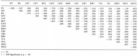
(click on image for a PDF version)
Initially, all possible combinations of up to six predictors were constituted. No more than six predictors were examined in any one model to insure no greater than a 10% ratio of predictors to observations (i.e., to avoid overfitting the data). Since the analyses were for exploratory as well as predictive purposes, a family of models was examined rather than searching for a particular model. The family of models was initially chosen on the basis of the highest R square. Subsequently, models were compared with regard to their F ratios, PRESS statistics, coefficient significance, and variance inflation factors (Draper and Smith, 1981; Montgomery and Peck, 1982).
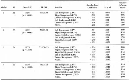
The best models for the sectioned (left, center, and right vegetation) variables are presented in Table 5.3, and the best models for the unsectioned (total area) variables are presented in Table 5.4. The sectioned and unsectioned variables were analyzed separately, since the latter are a linear combination of the former.
Table 5.3. Best regression models for sectioned variables.
(click on image for a PDF version)
Table 5.4. Best regression models for unsectioned variables.
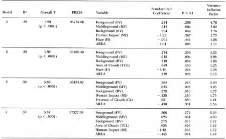
(click on image for a PDF version)
In general, it appears that breaking down the scenes and using measurements from left, center, and right sections improved the predictive power of the models. The R-square value from the best six-predictor unsectioned model was 0.39 (p <.0001), while for the best six-predictor section model the R-square was 0.5 (p <.0001). Among the findings for the sectioned models, it is interesting to note that LFV and RFV consistently appear as significant predictors of scenic beauty. Foreground vegetation might have been considered irrelevant to the perceived quality of scenic vistas or overlooks unless it simply blocked the vista, but this was not the case. In addition, the regression models for the sectioned variable (see Table 5.3) suggest that there does seem to be a preferred composition. Middle and background vegetation are preferred in the center, and foreground vegetation has an impact on the sides. It should be noted, however, that total foreground vegetation was not a significant predictor of scenic beauty. An examination of the signs of the regression weights for RFV and LFV suggests an explanation for this finding; RFV has a positive weight while LFV has a negative one, indicating that they nullified each other with regard to the overall effect of foreground vegetation on scenic beauty.
The stability of the signs of the regression weights for LFV and RFV was assessed by recalculating models with those two variables eight times while substituting other variables into the model with RFV and LFV. The regression weight signs and their significance were stable across all trials. Thus, the signs of the coefficients for RFV and LFV were not spurious functions of other variables present in the models. However, it is also conceivable that the countervailing signs of LFV and RFV are a result of a suppressor relationship between these two variables. An examination of the correlation matrix (see Table 5.2) does, in fact, suggest such a possibility. In this case both right and left foreground vegetation are negatively correlated with scenic beauty while being positively correlated with one another.
In addition, the zero order correlation between RFV and SBE is not significant (p >0.05). Thus, the change in the RFV regression sign could indicate that LFV and RFV are mutually inhibiting nonpredictive variances. If this is indeed the case, and not a function of other variables, then the relationship should emerge even when no other variables are present in the regression equation. To test this hypothesis, SBE was regressed on LFV and RFV alone. The results of this computation are equivocal but do indicate that any suppression effect between these two predictors is relatively weak. The regression weight signs are the same as in the other equations (standardized coefficients are -0.68 and 0.30 for LFV and RFV, respectively), but the significance test on the RFV regression weight is not significant (p > 0.05).
Further supporting the assertion that any suppressor effects are weak are the multicollinearity diagnostics reported in Table 5.3. The variance inflation factors in all models are well below prescribed standards (see Belsley et al., 1980; Montgomery and Peck, 1982), indicating that multicollinearity, of which suppression is a special case, is not problematic.
It also seemed possible that the differences in signs of the regression weights for RFV and LFV could reflect differences in the distribution of amount of foreground vegetation between the left and right sections in the landscape scenes. Inspection of the means (10.10 and 9.39) and standard deviations (5.89 and 5.33) for LFV and RFV, respectively, suggests that this was not the case.
It is conceivable that right and left foreground vegetation differed in ways not adequately assessed by the measures used in this study. For example, it is possible that the type of vegetation (e.g., coniferous versus deciduous) is not evenly dispersed over right and left foreground. The landscape scenes were visually inspected for obvious content differences (i.e., factors such as shape or form, or the presence of coniferous versus deciduous vegetation) once by two of the co-authors and once independently by a third co-author. However, no apparent differences were detected simply by visual inspection.
As noted in Part I of this chapter, previous research (Buhyoff et al., 1982) has suggested a nonmonotonic relationship between perceived scenic beauty and the area of sharp mountains in a scene. The reason for this is unclear. One possibility may be that the greater the area taken up by background, the farther those elements are from the viewer. Consequently, they may lose positive visual qualities associated with scenic beauty, such as detail and texture. In the present study it was hypothesized that such a nonmonotonic relationship might represent the pattern of covariation between total background vegetation and scenic beauty as well. Visual inspection of the plot of residual SBE values versus total background area suggested that such a curvilinearity might be present. To test this, a regression analysis was done on one of the sets of total variables, including total background area (BV), while adding a total background area squared (BV2) term to the model to test the quadratic effect. Both BV and BV2 were significant predictors of scenic beauty (standardized b = 1.21, p <.0003 and b = -1.07, p < .0007, respectively), suggesting that both linear and nonmonotonic, nonlinear relationships are present in the data.
The findings of the experiment suggest that landscape elements that are general with regard to their content (e.g., amount of background vegetation) are significant predictors of perceived scenic beauty. In addition, the spatial arrangement of these elements was a factor in the prediction of scenic beauty. However, other variables, including various measures of clouds and the presence of haze and human impact, were not predictive. The lack of relationship between these latter variables and perceived scenic beauty may be a function of restriction of range (i.e, extreme values on the continuum were not represented in this sample) or lack of measurement sensitivity. For example, in our sample of scenes, human impact tended to be in the background and was not predominant in the scene. In contrast, prior research has revealed significant effects when human artifacts are primary elements in the scene (Kaplan et al., 1972).
To better understand the nature of the differential weighting of left and right foreground in the prediction of perceived scenic beauty, a second experiment was conducted. The question addressed by this second experiment was whether differential preference for the left and right foreground of the image was a function of image content or was due to a perceptual bias resulting from hemispheric brain specialization (Gazzaniga, 1970; Harcum, 1978). A clear consensus among psychologists concerning the left-right bias has not been reached (Harcum 1978; Heron, 1957; Wickelgren, 1967; Gazzaniga, 1970; Gur et al., 1975).
In the present study, if such a right-left bias persists in monochotic presentations, it is conceivable that differential perception might result. Furthermore, since the majority of the population can be characterized by left side brain specialization (perceptual right side emphasis), right side preference might emerge in a random sample drawn from the population. This bias can be tested by simply reversing the image of the landscape (i.e., by turning the slide around) so that the content on the right side would now appear on the left, and vice versa. If the opposing regression weights are due to the specific content of the image, the new regression weight signs should be opposite to those in study 1. That is, LFV should change from negative to positive, and RFV should shift from positive to negative. If, on the other hand, the opposing regression weights are due to perceptual bias, such as differential processing of information from the left and right fields of vision, it would be expected that the regression weight signs for left and right foreground would remain stable.
In a separate experiment, 39 introductory psychology students at Virginia Polytechnic Institute and State University rated the reversed slides. None of these students had participated in the first study. SBE's were calculated and analyzed as before. The prediction models developed in this study were less successful than in the first one, with average R-square values of 0.36 as compared to 0.53 in the original models. The hypothesized left-right perceptual bias was not found. When the slides were reversed, preferences tended to be reversed as well. Thus, preference appears to be related to content rather than placement of foreground vegetation. In addition, the correlation between the SBE's from the original and the second study was only 0.83 (p < .0001), somewhat lower than expected on the basis of previous research, and background vegetation was not a significant predictor of scenic quality.
Conclusions and Recommendations
The present findings support previous work (Shafer et al., 1969; Brush and Palmer, 1979) which demonstrated the ability of general content classes of vegetation to predict scenic beauty. Of particular interest is the finding that foreground vegetation can have a substantial impact on the perceived scenic beauty of vistas. Unfortunately, the nature of this impact is complex, as indicated by both the differential regression weights found for LFV and RFV and the lack of impact of total foreground vegetation. There was no support for the notion that a perceptual left-right bias was responsible for the differential weights of LFV and RFV.
The stability of the weights for foreground vegetation suggests that particular foreground content and its placement within a scene are significant predictors of scenic quality. It is puzzling that, while viewers perceive specific content (i.e., left and right foreground) positively or negatively no matter what side of the image it is on, the correlation between SBE's for the original and reversed scenes was only 0.83. This suggests that the perceived quality of the original and reversed scenes is similar but far from identical.
Until the basis for the differential effects of LFV and RFV is better understood, it is difficult to make specific recommendations for management actions. It would obviously be unwise to generalize from the weights found here for left and right foreground to suggest left foreground be inhibited and right foreground be enhanced for any particular scenic overlook. In addition, as Weinstein (1976) has noted, the generalizability of any prediction model must be established by demonstrating its accuracy in other contexts. Thus, the efficacy and utility of these predictors must be evaluated for other sets of landscape scenes and other samples of observers.
The regression models examined in the present study explained a respectable but moderate amount of criterion variance. Nonetheless, a considerable amount of variance in the SBE's went unaccounted for. Given that the findings regarding LFV and RFV remain enigmatic, it may be that other relevant variables or attributes of the scenes went unrecognized, and that these variables may have been able to account for more of the SBE variance. That is, the variables used in these studies (e.g., LFV and RFV) may have been surrogates for these other, unrecognized variables.
The nature of these "other" variables remains unclear, but more complex formulations of environmental attributes must be considered as one variable alternative. Relatively abstract transactional constructs such as complexity, congruity, and mystery have been used effectively in research on environmental aesthetics (Wohlwill, 1968, 1976; Kaplan et al., 1972; Kaplan, 1973, 1975; Wohlwill and Harris, 1980; Feimer et al., 1981; Feimer, 1983), suggesting that a more holistic characterization of the relationships among the elements within the scene may add to prediction beyond that achieved in a simple and gross representation of content.
On a similar but somewhat less abstract plane, it is also conceivable that a more discriminating analysis of content, including an examination of vegetation type and visually salient physical attributes such as shape, form, and color, might add to predictive power. In any case, examination of these other classes of variables in conjunction with the kinds of variables used in this study holds promise for providing insight into the complex pattern of relationships that characterize aesthetic responses to natural settings.
Beyond demonstrating to managers and landscape architects that foreground does matter to visitors, we would like to offer several other observations based on our broader research program.
This research has focused on the foreground vegetation extant at parkway vistas. We have not studied the visual impacts of vegetation manipulation. For example, if controlled burns are used to eradicate unwanted woody plants, there may well be a severe, if temporary, reduction in overall scenic beauty. If mechanical means are used to reduce brushy vegetation, it is advisable to remove the cuttings since all research has demonstrated negative visual impacts from dead and down wood. Obviously, these suggestions must be interpreted in terms of other criteria, in addition to scenic beauty. For example, if herbicides are used, visitors may object to what they see as poisoning of the environment. Considerations of cost, nutrient cycling, erosion control, and other matters may lead to a choice of management actions that are scenically non-optimal. If this is the case, managers are advised to provide interpretation to the visitors to explain the necessity and temporary nature of the environmental disruption.
One of the major conclusions from our research over the years is that visual effects do not increase or decrease steadily with changes in the physical environment. Instead, scenic beauty often behaves in a marginal utility manner. A small amount of damage, for example, causes rapid declines in perceived scenic beauty, after which additional damage has little negative effect. Therefore, it is possible that a small amount of vegetation management on certain vistas might significantly raise their scenic beauty, while extensive and costly work at heavily overgrown sites may provide little improvement in visitor satisfaction. While we cannot be more specific in our suggestions, we would advise parkway management to inventory vista scenic resources to determine sites where investment in vegetation management might provide the greatest returns.
A second general suggestion emerging from our research is that in scenic beauty, one can have "too much of a good thing." As noted in Part I of this chapter, jagged mountains and large urban trees contribute to scenic beauty but apparently only up to some point, after which additional increments lead to declines in scenic beauty. As to foreground vegetation on the Blue Ridge Parkway, as a general rule the more open the vista the better. However, carried to an extreme, this management guideline might well be counter-productive. A certain amount of foreground vegetation provides vista framing or perhaps is attractive in itself, as with flowering shrubs or plants that attract birds. Lawn-like vista foregrounds might be viewed as unnatural, and this might become even more of a liability if public preference for unmodified nature increases in the future. Some mixture of enclosed and open vistas might be sought in an effort to promote landscape diversity, generally regarded as central to quality visual experiences.
Finally, decisions about vista vegetation management should be framed within the larger context of the Blue Ridge Parkway visual environment and visitor behavior. Whether or not encroaching foreground vegetation at any one vista should be removed depends on the array of other vistas available in a region, and how "regions" are defined should be based in part on patterns of visitation.
In the final analysis, responsibility for making such choices rests with the managers. Science, such as that reported in this article, can support and inform managerial judgments, but it cannot replace it. To be successful, park and forest landscape management must take into account the unique blend of natural environmental features, man-made developments, and visitor attitudes and behavior found at particular sites. Science seeks generalizable truths and necessarily simplifies the world to study it. At the same time, scientific research has the great strength of objectivity and the potential for altering the basic mindsets managers bring to their work. If public wildland resources are to produce the stream of social benefits they are capable of producing, managers and scientists must continue to seek ways of working together.
REFERENCES
Arthur, L.M. 1977. Predicting scenic beauty of forest environments: Some empirical tests. Forest Science 23(2): 151-160.
Belsley, D.A., E. Kuh, and R. E. Welsch. 1980. Regression Diagnostics...Identifying Influential Data and Sources of Collinearity. New York: John Wiley and Sons.
Brush, R.O., and J. F. Palmer. 1979. Measuring the impact of urbanization on scenic quality: Land use change in the northeast. Proceedings of Our National Landscape: A Conference on Applied Techniques for Analysis and Management of the Visual Resource. Berkeley, CA: USDA Forest Service, p. 358-364.
Buhyoff, G.J., L. K. Arndt, and D. B. Propst. 1981. Interval scaling of landscape preference by direct and indirect methods. Landscape Planning 8(3):257-267.
Buhyoff, G.J., L. Gauthier,, and J. D. Wellman. 1984. Predicting scenic quality for urban forests using vegetation measurements. Forest Science 30(1):71-82.
Buhyoff, G.J., and W. A. Leuschner. 1978. Estimating psychological disutility from damaged forest stands. Forest Science 24(2): 424-432.
Buhyoff, G.J., W. A. Leuschner, and L. K. Arndt. 1980. The replication of a scenic preference function. Forest Science 26(2): 227-230.
Buhyoff, G. J., and M. F. Riesenman. 1979. Experimental manipulation of dimensionality in landscape preference judgments: A quantitative validation. Leisure Sciences: An Interdisciplinary Journal 2(3): 221-238.
Buhyoff, G.J., and J. D. Wellman. 1979. Seasonality bias in landscape preference research. Leisure Sciences 2(2): 181-190
Buhyoff, G.J., and J. D. Wellman. 1979. The specification of a non-linear psychophysical function for visual landscape dimensions. Journal of Leisure Research 12(3): 157-172.
Buhyoff, G.J., J. D. Wellman, H. Harvey, and R. A. Fraser. 1978. Landscape architects' interpretations of people's landscape preferences. Journal of Environmental Management 6(3): 255-262.
Buhyoff, G.J., J. D. Wellman, and T. C. Daniel. 1982. Predicting scenic quality for mountain pine beetle and western spruce budworm damaged forest vistas. Forest Science 28(4): 827-838.
Daniel, T.C., and R.C. Boster. 1976. Measuring landscape esthetics; scenic beauty estimation method. USDA Forest Service, Rocky Mtn. Forest and Range Experiment Station. Fort Collins, CO. 66pp.
Draper, N.R., and H. Smith. 1981. Applied Regression Analysis. New York: John Wiley and Sons.
Ebel, R.L. 1981. Estimation of the reliability of ratings. Psychometrica 16:407-423.
Feimer, N.R. 1983. Environmental perception and cognition in rural contexts. In A.W. Childs and G.B. Mellon (Eds.), Rural Psychology. New York: Plenum Press, 113-149.
Feimer N.R., R.C. Smardon, and K.H. Craik. 1981. Evaluating the effectiveness of observer-based visual resource and impact assessment methods. Landscape Research 6: 12-16.
Gauthier, Laureen J. 1981. An Investigation of Preferences for Urban Vegetation through Multidimensional and Unidimensional scaling techniques. M.S. Thesis. Virginia Polytechnic Institute and State University, Blacksburg, VA. 191 pp.
Gazzaniga, M.S. 1970. The Bisected Brain. New York: Appleton.
Green, D.M., and J. A. Swetts. 1966. Signal Detection and Psychophysics. New York: John Wiley and Sons.
Guilford, J.P. 1954. Psychometric Methods. New York: McGraw-Hill.
Gur, R.E., R. C. Gur, and B. Marshalek. 1975. Classroom seating and functional brain asymmetry. Journal of Educational Psychology 67: 151-153.
Harcum, E.R. 1978. Lateral dominance as a determinant of temporal order of responding. In M. Kinsbourne (Ed.) Assymetrical Function of the Brain. Cambridge: Cambridge University Press.
Harvey, H. 1977. Landscape Preference Quantification: A Comparison of Methods. Unpublished M.S. Thesis, Virginia Polytechnic Institute and State University, Blacksburg, VA. 110pp.
Heron, W. 1957. Perception as a function of retinal locus and attention. American Journal of Psychology 70: 38-48.
Hull, R. Bruce, IV. 1984. Simulation and Evaluation of Scenic Beauty Temporal Distributions in Southern Pine Stands. Ph.D. Dissertation, Virginia Polytechnic Institute and State University, Blacksburg, VA. 159p.
Hull, R.B., G. J. Buhyoff, and T. C. Daniel. 1984. Measurement of scenic beauty: the law of comparative judgment and scenic beauty estimation procedures. Forest Science 30(4): 1084-1096.
Kaplan, R. 1973. Predictors of environmental preference: Designers and clients. In W.F.E. Preiser (Ed.) Environmental Design Research. Stroudsburg, PA: Dowden, Hutchinson & Ross.
Kaplan, R. 1975. Some methods and strategies in the prediction of preference. In E.H. Zube, R.O. Brush, and J.G. Fabos (Eds.), Landscape Assessment: Values, Perceptions, and Resources. Stroudsburg, PA: Dowden, Hutchinson, and Ross.
Kaplan, S., R. Kaplan, and J. S. Wendt. 1972. Rated preference and complexity for natural and urban visual materials. Perception and Psychophysics 12:354-356.
Lien, J.N., G. J. Buhyoff, and J. D. Wellman. 1984. Development and operationalization of visual preference models for urban forest management. Final Report. U.S.D.A. Forest Service, North Central Forest Experiment Station. Chicago, IL. 32p.
Montgomery, D. C., and E. A. Peck. 1982. Introduction to Linear Regression Analysis. New York: John Wiley & Sons.
Patsfall, M. R., N. R. Feimer, G. J. Buhyoff, and J. D. Wellman. 1984. The prediction of scenic beauty from landscape content and composition. Journal of Environmental psychology 11: 7-26.
Propst, D. B., and G. J. Buyoff. 1981. Policy capturing and landscape preference quantification: a methodological study. Journal of Environmental Management 11: 45-59.
Shafer, E.L., Jr., J. F. Hamilton, Jr., and E. A. Schmidt. 1969. Natural landscape preferences: a predictive mode. Journal of Leisure Research 1(1):1-10.
Thurstone, L.L. 1927. A law of comparative judgment. Psychological Review 34: 273-286.
Togerson, W. S. 1958. Theory and Methods of Scaling. New York: Wiley.
Vodak, M. C., P. L. Roberts, J. D. Wellman, and G. J. Buyoff. 1985. Scenic impacts of eastern hardwood management. Forest Science 31(2): 289-301.
Weinstein, N. D. 1976. The statistical prediction of environmental preferences. Environment and Behavior 8: 611-626.
Wickelgren, L.W. 1967. Convergence in the human newborn. Journal of Experimental Child Psychology 5: 74-85.
Wohlwill, J.F. 1968. Amount of stimulus exploration and preference as differential functions of stimulus complexity. Preference and Psychophysics 4:307-312.
Wohlwill, J.F. 1976. Environmental aesthetics: the environment as a source of affect. In I. Altman and J.F. Wohnwill (Eds.). Human Behavior and Environment: Advances in Theory and Research. Vol. 1. New York: Plenum Press.
Wohlwill, J.F., and G. Harris. 1980. Response to congruity or contrast for man-made features in natural recreation settings. Leisure Sciences 3: 349-365.
Zube, E. 1976. Perception of landscape and land use. In I. Altman and J.F. Wohlwill (Eds.). Human Behavior and Environment: Advances in Theory and Research. Vol. 1. New York: Plenum Press.
Zube, E.H., J. L. Sells, and J. G. Taylor. 1982. Landscape perception: research, application and theory. Landscape Planning 9:1-33.
| <<< Previous | <<< Contents >>> | Next >>> |
chap5.htm
Last Updated: 06-Dec-2007